12  Data Grouping and Aggregation

Grouping and aggregation are essential in data science because they enable meaningful analysis and insights from complex and large-scale datasets. Here are key reasons why they are important:

• Data Summarization: Grouping allows you to condense large amounts of data into concise summaries. Aggregation provides statistical summaries (e.g., mean, sum, count), making it easier to understand data trends and characteristics without needing to examine every detail.
• Insights Across Categories: Grouping by categories, like regions, demographics, or time periods, lets you analyze patterns within each group. For example, aggregating sales data by region can reveal which areas are performing better, or grouping customer data by age group can highlight consumer trends.
• Time Series Analysis: In time-series data, grouping by time intervals (e.g., day, month, quarter) allows you to observe trends over time, which can be crucial for forecasting, seasonal analysis, and trend detection.
• Reducing Data Complexity: By summarizing data at a higher level, you reduce complexity, making it easier to visualize and interpret, especially in large datasets where working with raw data could be overwhelming.

In this chapter, we are going to see grouping and aggregating using pandas. Grouping and aggregating will help to achieve data analysis easily using various functions. These methods will help us to the group and summarize our data and make complex analysis comparatively easy.

Througout this chapter, we will use gdp_lifeExpectancy.csv, let’s read the csv file to pandas dataframe first

import pandas as pd
import numpy as np
import seaborn as sns
import matplotlib.pyplot as plt

%matplotlib inline

# Load the data
gdp_lifeExp_data = pd.read_csv('./Datasets/gdp_lifeExpectancy.csv')
gdp_lifeExp_data.head()

	country	continent	year	lifeExp	pop	gdpPercap
0	Afghanistan	Asia	1952	28.801	8425333	779.445314
1	Afghanistan	Asia	1957	30.332	9240934	820.853030
2	Afghanistan	Asia	1962	31.997	10267083	853.100710
3	Afghanistan	Asia	1967	34.020	11537966	836.197138
4	Afghanistan	Asia	1972	36.088	13079460	739.981106

12.1 Grouping by a single column

groupby() allows you to split a DataFrame based on the values in one or more columns. First, we’ll explore grouping by a single column.

12.1.1 Syntax of groupby()

• DataFrame.groupby(by="column_name") – Groups data by the specified column.

Consider the life expectancy dataset. suppose we want to group by the observations by continent by passing it as an argument to the groupby() method.

#Creating a GroupBy object
grouped = gdp_lifeExp_data.groupby('continent')
#This will split the data into groups that correspond to values of the column 'continent'

The groupby() method returns a GroupBy object.

#A 'GroupBy' objects is created with the `groupby()` function
type(grouped)

pandas.core.groupby.generic.DataFrameGroupBy

The GroupBy object grouped contains the information of the groups in which the data is distributed. Each observation has been assigned to a specific group of the column(s) used to group the data. However, note that the dataset is not physically split into different DataFrames. For example, in the above case, each observation is assigned to a particular group depending on the value of the continent for that observation. However, all the observations are still in the same DataFrame data.

12.1.2 Attributes and methods of the GroupBy object

12.1.2.1 keys

The object(s) grouping the data are called key(s). Here continent is the group key. The keys of the GroupBy object can be seen using Its keys attribute.

#Key(s) of the GroupBy object
grouped.keys

'continent'

12.1.2.2 ngroups

The number of groups in which the data is distributed based on the keys can be seen with the ngroups attribute.

#The number of groups based on the key(s)
grouped.ngroups

5

The group names are the keys of the dictionary, while the row labels are the corresponding values

#Group names
grouped.groups.keys()

dict_keys(['Africa', 'Americas', 'Asia', 'Europe', 'Oceania'])

12.1.2.3 groups

The groups attribute of the GroupBy object contains the group labels (or names) and the row labels of the observations in each group, as a dictionary.

#The groups (in the dictionary format)
grouped.groups

{'Africa': [24, 25, 26, 27, 28, 29, 30, 31, 32, 33, 34, 35, 36, 37, 38, 39, 40, 41, 42, 43, 44, 45, 46, 47, 120, 121, 122, 123, 124, 125, 126, 127, 128, 129, 130, 131, 156, 157, 158, 159, 160, 161, 162, 163, 164, 165, 166, 167, 192, 193, 194, 195, 196, 197, 198, 199, 200, 201, 202, 203, 204, 205, 206, 207, 208, 209, 210, 211, 212, 213, 214, 215, 228, 229, 230, 231, 232, 233, 234, 235, 236, 237, 238, 239, 252, 253, 254, 255, 256, 257, 258, 259, 260, 261, 262, 263, 264, 265, 266, 267, ...], 'Americas': [48, 49, 50, 51, 52, 53, 54, 55, 56, 57, 58, 59, 132, 133, 134, 135, 136, 137, 138, 139, 140, 141, 142, 143, 168, 169, 170, 171, 172, 173, 174, 175, 176, 177, 178, 179, 240, 241, 242, 243, 244, 245, 246, 247, 248, 249, 250, 251, 276, 277, 278, 279, 280, 281, 282, 283, 284, 285, 286, 287, 300, 301, 302, 303, 304, 305, 306, 307, 308, 309, 310, 311, 348, 349, 350, 351, 352, 353, 354, 355, 356, 357, 358, 359, 384, 385, 386, 387, 388, 389, 390, 391, 392, 393, 394, 395, 432, 433, 434, 435, ...], 'Asia': [0, 1, 2, 3, 4, 5, 6, 7, 8, 9, 10, 11, 84, 85, 86, 87, 88, 89, 90, 91, 92, 93, 94, 95, 96, 97, 98, 99, 100, 101, 102, 103, 104, 105, 106, 107, 216, 217, 218, 219, 220, 221, 222, 223, 224, 225, 226, 227, 288, 289, 290, 291, 292, 293, 294, 295, 296, 297, 298, 299, 660, 661, 662, 663, 664, 665, 666, 667, 668, 669, 670, 671, 696, 697, 698, 699, 700, 701, 702, 703, 704, 705, 706, 707, 708, 709, 710, 711, 712, 713, 714, 715, 716, 717, 718, 719, 720, 721, 722, 723, ...], 'Europe': [12, 13, 14, 15, 16, 17, 18, 19, 20, 21, 22, 23, 72, 73, 74, 75, 76, 77, 78, 79, 80, 81, 82, 83, 108, 109, 110, 111, 112, 113, 114, 115, 116, 117, 118, 119, 144, 145, 146, 147, 148, 149, 150, 151, 152, 153, 154, 155, 180, 181, 182, 183, 184, 185, 186, 187, 188, 189, 190, 191, 372, 373, 374, 375, 376, 377, 378, 379, 380, 381, 382, 383, 396, 397, 398, 399, 400, 401, 402, 403, 404, 405, 406, 407, 408, 409, 410, 411, 412, 413, 414, 415, 416, 417, 418, 419, 516, 517, 518, 519, ...], 'Oceania': [60, 61, 62, 63, 64, 65, 66, 67, 68, 69, 70, 71, 1092, 1093, 1094, 1095, 1096, 1097, 1098, 1099, 1100, 1101, 1102, 1103]}

12.1.2.4 groups.values

The groups.values attribute of the GroupBy object contains the row labels of the observations in each group, as a dictionary.

#Group values are the row labels corresponding to a particular group
grouped.groups.values()

dict_values([Index([  24,   25,   26,   27,   28,   29,   30,   31,   32,   33,
       ...
       1694, 1695, 1696, 1697, 1698, 1699, 1700, 1701, 1702, 1703],
      dtype='int64', length=624), Index([  48,   49,   50,   51,   52,   53,   54,   55,   56,   57,
       ...
       1634, 1635, 1636, 1637, 1638, 1639, 1640, 1641, 1642, 1643],
      dtype='int64', length=300), Index([   0,    1,    2,    3,    4,    5,    6,    7,    8,    9,
       ...
       1670, 1671, 1672, 1673, 1674, 1675, 1676, 1677, 1678, 1679],
      dtype='int64', length=396), Index([  12,   13,   14,   15,   16,   17,   18,   19,   20,   21,
       ...
       1598, 1599, 1600, 1601, 1602, 1603, 1604, 1605, 1606, 1607],
      dtype='int64', length=360), Index([  60,   61,   62,   63,   64,   65,   66,   67,   68,   69,   70,   71,
       1092, 1093, 1094, 1095, 1096, 1097, 1098, 1099, 1100, 1101, 1102, 1103],
      dtype='int64')])

12.1.2.5 size()

The size() method of the GroupBy object returns the number of observations in each group.

#Number of observations in each group
grouped.size()

continent
Africa      624
Americas    300
Asia        396
Europe      360
Oceania      24
dtype: int64

12.1.2.6 first()

The first non missing element of each group is returned with the first() method of the GroupBy object.

#The first element of the group can be printed using the first() method
grouped.first()

	country	year	lifeExp	pop	gdpPercap
continent
Africa	Algeria	1952	43.077	9279525	2449.008185
Americas	Argentina	1952	62.485	17876956	5911.315053
Asia	Afghanistan	1952	28.801	8425333	779.445314
Europe	Albania	1952	55.230	1282697	1601.056136
Oceania	Australia	1952	69.120	8691212	10039.595640

12.1.2.7 get_group()

This method returns the observations for a particular group of the GroupBy object.

#Observations for individual groups can be obtained using the get_group() function
grouped.get_group('Asia')

	country	continent	year	lifeExp	pop	gdpPercap
0	Afghanistan	Asia	1952	28.801	8425333	779.445314
1	Afghanistan	Asia	1957	30.332	9240934	820.853030
2	Afghanistan	Asia	1962	31.997	10267083	853.100710
3	Afghanistan	Asia	1967	34.020	11537966	836.197138
4	Afghanistan	Asia	1972	36.088	13079460	739.981106
...	...	...	...	...	...	...
1675	Yemen, Rep.	Asia	1987	52.922	11219340	1971.741538
1676	Yemen, Rep.	Asia	1992	55.599	13367997	1879.496673
1677	Yemen, Rep.	Asia	1997	58.020	15826497	2117.484526
1678	Yemen, Rep.	Asia	2002	60.308	18701257	2234.820827
1679	Yemen, Rep.	Asia	2007	62.698	22211743	2280.769906

396 rows × 6 columns

12.2 Data aggregation within groups

12.2.1 Common Aggregation Functions

Aggregation functions are essential for summarizing and analyzing data in pandas. These functions allow you to compute summary statistics for your data, making it easier to identify trends and patterns.

Below are some of the most commonly used aggregation functions when working with grouped data in pandas:

• mean() – Calculates the average value of the group.
• sum() – Computes the total value by summing all elements in the group.
• min() – Finds the minimum value in the group.
• max() – Finds the maximum value in the group.
• count() – Returns the number of occurrences or entries in the group.
• median() – Finds the middle value in the sorted group.
• std() – Calculates the standard deviation, measuring the spread or variation in the values of the group.

Each of these functions can help summarize and provide insights into different aspects of the grouped data.

Consider the life expectancy dataset, let’s find the mean life expectancy, population and GDP per capita for each country during the period of 1952 -2007.

Next, we’ll find the mean statistics for each group with the mean() method. The method will be applied on all columns of the DataFrame and all groups.

#Grouping the observations by 'country'
grouped_country = gdp_lifeExp_data.drop (['continent', 'year'], axis = 1).groupby('country')

#Finding the mean stastistic of all columns of the DataFrame and all groups
grouped_country.mean()

	lifeExp	pop	gdpPercap
country
Afghanistan	37.478833	1.582372e+07	802.674598
Albania	68.432917	2.580249e+06	3255.366633
Algeria	59.030167	1.987541e+07	4426.025973
Angola	37.883500	7.309390e+06	3607.100529
Argentina	69.060417	2.860224e+07	8955.553783
...	...	...	...
Vietnam	57.479500	5.456857e+07	1017.712615
West Bank and Gaza	60.328667	1.848606e+06	3759.996781
Yemen, Rep.	46.780417	1.084319e+07	1569.274672
Zambia	45.996333	6.353805e+06	1358.199409
Zimbabwe	52.663167	7.641966e+06	635.858042

142 rows × 3 columns

Next, we’ll find the standard deviation statistics for each group with the std() method.

grouped_country.std()

	lifeExp	pop	gdpPercap
country
Afghanistan	5.098646	7.114583e+06	108.202929
Albania	6.322911	8.285855e+05	1192.351513
Algeria	10.340069	8.613355e+06	1310.337656
Angola	4.005276	2.672281e+06	1165.900251
Argentina	4.186470	7.546609e+06	1862.583151
...	...	...	...
Vietnam	12.172331	2.052585e+07	567.482251
West Bank and Gaza	11.000069	1.023057e+06	1716.840614
Yemen, Rep.	11.019302	5.590408e+06	609.939160
Zambia	4.453246	3.096949e+06	247.494984
Zimbabwe	7.071816	3.376895e+06	133.689213

142 rows × 3 columns

Alternatively, you can compute other statistical metrics.

12.2.2 Multiple aggregations and Custom aggregation using agg()

12.2.2.1 Multiple aggregations

Directly applying the aggregate methods of the GroupBy object such as mean, count, etc., lets us apply only one function at a time. Also, we may wish to apply an aggregate function of our own, which is not there in the set of methods of the GroupBy object, such as the range of values of a column.

The agg() function of a GroupBy object lets us aggregate data using:

1. Multiple aggregation functions

2. Custom aggregate functions (in addition to in-built functions like mean, std, count etc.)

Consider the life expectancy dataset, Let us use the agg() method of the GroupBy object to simultaneously find the mean and standard deviation of the gdpPercap for each country.

For aggregating by multiple functions, we pass a list of strings to agg(), where the strings are the function names.

grouped_country['gdpPercap'].agg(['mean','std']).sort_values(by = 'mean',ascending = False).head()

	mean	std
country
Kuwait	65332.910472	33882.139536
Switzerland	27074.334405	6886.463308
Norway	26747.306554	13421.947245
United States	26261.151347	9695.058103
Canada	22410.746340	8210.112789

12.2.2.2 Custom aggregation

In addition to the mean and standard deviation of the gdpPercap of each country, let us also include the range of gdpPercap in the table above using lambda function

grouped_country['gdpPercap'].agg(lambda x: x.max() - x.min())

country
Afghanistan            342.670088
Albania               4335.973390
Algeria               3774.359280
Angola                3245.635491
Argentina             6868.064587
                         ...     
Vietnam               1836.509912
West Bank and Gaza    5595.075290
Yemen, Rep.           1499.052330
Zambia                 705.723500
Zimbabwe               392.478061
Name: gdpPercap, Length: 142, dtype: float64

# define a function that calculates the range
def range_func(x):
    return x.max() - x.min()

# apply the range function to the 'gdpPercap' column besides the mean and standard deviation
grouped_country['gdpPercap'].agg(['mean', 'std', range_func]).sort_values(by = 'range_func', ascending = False)

	mean	std	range_func
country
Kuwait	65332.910472	33882.139536	85404.702920
Singapore	17425.382267	14926.147774	44828.041413
Norway	26747.306554	13421.947245	39261.768450
Hong Kong, China	16228.700865	12207.329731	36670.557461
Ireland	15758.606238	11573.311022	35465.716022
...	...	...	...
Rwanda	675.669043	142.229906	388.246772
Senegal	1533.121694	105.399353	344.572767
Afghanistan	802.674598	108.202929	342.670088
Ethiopia	509.115155	96.427627	328.659296
Burundi	471.662990	99.329720	292.403419

142 rows × 3 columns

For aggregating by multiple functions & changing the column names resulting from those functions, we pass a list of tuples to agg(), where each tuple is of length two, and contains the new column name & the function to be applied.

#Simultaneous renaming of columns while grouping
grouped_country['gdpPercap'].agg([('Average','mean'),('Standard Deviation','std'),('90th Percentile',lambda x:x.quantile(0.9))]).sort_values(by = '90th Percentile',ascending = False)

	Average	Standard Deviation	90th Percentile
country
Kuwait	65332.910472	33882.139536	109251.315590
Norway	26747.306554	13421.947245	44343.894158
United States	26261.151347	9695.058103	38764.132898
Singapore	17425.382267	14926.147774	35772.742520
Switzerland	27074.334405	6886.463308	34246.394240
...	...	...	...
Liberia	604.814141	98.988329	706.275527
Malawi	575.447212	122.999953	689.590541
Burundi	471.662990	99.329720	615.597260
Myanmar	439.333333	175.401531	592.300000
Ethiopia	509.115155	96.427627	577.448804

142 rows × 3 columns

12.2.3 Multiple aggregate functions on multiple columns

Let us find the mean and standard deviation of lifeExp and pop for each country

# find the meand and standard deviation of the 'lifeExp' and 'pop' column for each country
grouped_country[['lifeExp', 'pop']].agg(['mean', 'std']).sort_values(by = ('lifeExp', 'mean'), ascending = False)

	lifeExp		pop
	mean	std	mean	std
country
Iceland	76.511417	3.026593	2.269781e+05	4.854168e+04
Sweden	76.177000	3.003990	8.220029e+06	6.365660e+05
Norway	75.843000	2.423994	4.031441e+06	4.107955e+05
Netherlands	75.648500	2.486363	1.378680e+07	2.005631e+06
Switzerland	75.565083	4.011572	6.384293e+06	8.582009e+05
...	...	...	...	...
Mozambique	40.379500	4.599184	1.204670e+07	4.457509e+06
Guinea-Bissau	39.210250	4.937369	8.820084e+05	3.132917e+05
Angola	37.883500	4.005276	7.309390e+06	2.672281e+06
Afghanistan	37.478833	5.098646	1.582372e+07	7.114583e+06
Sierra Leone	36.769167	3.937828	3.605425e+06	1.270945e+06

142 rows × 4 columns

12.2.4 Distinct aggregate functions on multiple columns

For aggregating by multiple functions, we pass a list of strings to agg(), where the strings are the function names.

For aggregating by multiple functions & changing the column names resulting from those functions, we pass a list of tuples to agg(), where each tuple is of length two, and contains the new column name as the first object and the function to be applied as the second object of the tuple.

For aggregating by multiple functions such that a distinct set of functions is applied to each column, we pass a dictionary to agg(), where the keys are the column names on which the function is to be applied, and the values are the list of strings that are the function names, or a list of tuples if we also wish to name the aggregated columns.

# We can use a list to apply multiple aggregation functions to a single column, and a dictionary to specify different functions for multiple columns
# Use string names for the aggregation functions
grouped_country.agg({"gdpPercap": ["mean", "std"], "lifeExp": ["median", "std"], "pop": ["max", "min"]})

	gdpPercap		lifeExp		pop
	mean	std	median	std	max	min
country
Afghanistan	802.674598	108.202929	39.1460	5.098646	31889923	8425333
Albania	3255.366633	1192.351513	69.6750	6.322911	3600523	1282697
Algeria	4426.025973	1310.337656	59.6910	10.340069	33333216	9279525
Angola	3607.100529	1165.900251	39.6945	4.005276	12420476	4232095
Argentina	8955.553783	1862.583151	69.2115	4.186470	40301927	17876956
...	...	...	...	...	...	...
Vietnam	1017.712615	567.482251	57.2900	12.172331	85262356	26246839
West Bank and Gaza	3759.996781	1716.840614	62.5855	11.000069	4018332	1030585
Yemen, Rep.	1569.274672	609.939160	46.6440	11.019302	22211743	4963829
Zambia	1358.199409	247.494984	46.0615	4.453246	11746035	2672000
Zimbabwe	635.858042	133.689213	53.1765	7.071816	12311143	3080907

142 rows × 6 columns

Next, for each country, find the mean and standard deviation of the lifeExp, and the minimum and maximum values of gdpPercap.

#Specifying arguments to the function as a dictionary if distinct functions are to be applied on distinct columns
grouped_country.agg({'lifeExp':[('Average','mean'),('Standard deviation','std')],'gdpPercap':['min','max']})

	lifeExp		gdpPercap
	Average	Standard deviation	min	max
country
Afghanistan	37.478833	5.098646	635.341351	978.011439
Albania	68.432917	6.322911	1601.056136	5937.029526
Algeria	59.030167	10.340069	2449.008185	6223.367465
Angola	37.883500	4.005276	2277.140884	5522.776375
Argentina	69.060417	4.186470	5911.315053	12779.379640
...	...	...	...	...
Vietnam	57.479500	12.172331	605.066492	2441.576404
West Bank and Gaza	60.328667	11.000069	1515.592329	7110.667619
Yemen, Rep.	46.780417	11.019302	781.717576	2280.769906
Zambia	45.996333	4.453246	1071.353818	1777.077318
Zimbabwe	52.663167	7.071816	406.884115	799.362176

142 rows × 4 columns

12.3 Grouping by Multiple Columns

Above, we demonstrated grouping by a single column, which is useful for summarizing data based on one categorical variable. However, in many cases, we need to group by multiple columns. Grouping by multiple columns allows us to create more detailed summaries by accounting for multiple categorical variables. This approach enables us to analyze data at a finer granularity, revealing insights that might be missed with single-column grouping alone.

12.3.1 Basic Syntax for Grouping by Multiple Columns

Use groupby() with a list of column names to group data by multiple columns.

• DataFrame.groupby(by=["col1", "col2"])

Consider the life expectancy dataset, we can group by both country and continent to analyze gdpPercap, lifeExp, and pop trends for each country within each continent, providing a more comprehensive view of the data.

#Grouping by multiple columns
grouped_continent_contry = gdp_lifeExp_data.groupby(['continent', 'country'])[ "lifeExp"].agg(['mean', 'std', 'max', 'min']).sort_values(by = 'mean', ascending = False)

grouped_continent_contry

		mean	std	max	min
continent	country
Europe	Iceland	76.511417	3.026593	81.757	72.490
	Sweden	76.177000	3.003990	80.884	71.860
	Norway	75.843000	2.423994	80.196	72.670
	Netherlands	75.648500	2.486363	79.762	72.130
	Switzerland	75.565083	4.011572	81.701	69.620
...	...	...	...	...	...
Africa	Mozambique	40.379500	4.599184	46.344	31.286
	Guinea-Bissau	39.210250	4.937369	46.388	32.500
	Angola	37.883500	4.005276	42.731	30.015
Asia	Afghanistan	37.478833	5.098646	43.828	28.801
Africa	Sierra Leone	36.769167	3.937828	42.568	30.331

142 rows × 4 columns

12.3.2 Understanding Hierarchical (Multi-Level) Indexing

• Grouping by multiple columns creates a hierarchical index (also called a multi-level index).
• This index allows each level (e.g., continent, country) to act as an independent category that can be accessed individually.

In the above output, continent and country form a two-level hierarchical index, allowing us to drill down from continent-level to country-level summaries.

grouped_continent_contry.index.nlevels

2

# get the first level of the index
grouped_continent_contry.index.levels[0]

Index(['Africa', 'Americas', 'Asia', 'Europe', 'Oceania'], dtype='object', name='continent')

# get the second level of the index
grouped_continent_contry.index.levels[1]

Index(['Afghanistan', 'Albania', 'Algeria', 'Angola', 'Argentina', 'Australia',
       'Austria', 'Bahrain', 'Bangladesh', 'Belgium',
       ...
       'Uganda', 'United Kingdom', 'United States', 'Uruguay', 'Venezuela',
       'Vietnam', 'West Bank and Gaza', 'Yemen, Rep.', 'Zambia', 'Zimbabwe'],
      dtype='object', name='country', length=142)

12.3.3 Subsetting Data in a Hierarchical Index

grouped_continent_country is still a DataFrame with hierarchical indexing. You can use .loc[] for subsetting, just as you would with a single-level index.

# get the observations for the 'Americas' continent
grouped_continent_contry.loc['Americas'].head()

	mean	std	max	min
country
Canada	74.902750	3.952871	80.653	68.750
United States	73.478500	3.343781	78.242	68.440
Puerto Rico	72.739333	3.984267	78.746	64.280
Cuba	71.045083	6.022798	78.273	59.421
Uruguay	70.781583	3.342937	76.384	66.071

# get the mean life expectancy for the 'Americas' continent
grouped_continent_contry.loc['Americas']['mean'].head()

country
Canada           74.902750
United States    73.478500
Puerto Rico      72.739333
Cuba             71.045083
Uruguay          70.781583
Name: mean, dtype: float64

# another way to get the mean life expectancy for the 'Americas' continent
grouped_continent_contry.loc['Americas', 'mean'].head()

country
Canada           74.902750
United States    73.478500
Puerto Rico      72.739333
Cuba             71.045083
Uruguay          70.781583
Name: mean, dtype: float64

You can use a tuple to access data for specific levels in a multi-level index.

# get the observations for the 'United States' country
grouped_continent_contry.loc[( 'Americas', 'United States')]

mean    73.478500
std      3.343781
max     78.242000
min     68.440000
Name: (Americas, United States), dtype: float64

grouped_continent_contry.loc[( 'Americas', 'United States'), ['mean', 'std']]

mean    73.478500
std      3.343781
Name: (Americas, United States), dtype: float64

gdp_lifeExp_data.columns

Index(['country', 'continent', 'year', 'lifeExp', 'pop', 'gdpPercap'], dtype='object')

Finally, you can use reset_index() to convert the hierarchical index into a regular index, allowing you to apply the standard subsetting and filtering methods covered in previous chapters

grouped_continent_contry.reset_index().head()

	continent	country	mean	std	max	min
0	Europe	Iceland	76.511417	3.026593	81.757	72.49
1	Europe	Sweden	76.177000	3.003990	80.884	71.86
2	Europe	Norway	75.843000	2.423994	80.196	72.67
3	Europe	Netherlands	75.648500	2.486363	79.762	72.13
4	Europe	Switzerland	75.565083	4.011572	81.701	69.62

12.3.4 Grouping by multiple columns and aggregating multiple variables

#Grouping by multiple columns
grouped_continent_contry_multi = gdp_lifeExp_data.groupby(['continent', 'country','year'])[ ['lifeExp', 'pop', 'gdpPercap']].agg(['mean', 'max', 'min'])
grouped_continent_contry_multi

			lifeExp			pop			gdpPercap
			mean	max	min	mean	max	min	mean	max	min
continent	country	year
Africa	Algeria	1952	43.077	43.077	43.077	9279525.0	9279525	9279525	2449.008185	2449.008185	2449.008185
		1957	45.685	45.685	45.685	10270856.0	10270856	10270856	3013.976023	3013.976023	3013.976023
		1962	48.303	48.303	48.303	11000948.0	11000948	11000948	2550.816880	2550.816880	2550.816880
		1967	51.407	51.407	51.407	12760499.0	12760499	12760499	3246.991771	3246.991771	3246.991771
		1972	54.518	54.518	54.518	14760787.0	14760787	14760787	4182.663766	4182.663766	4182.663766
...	...	...	...	...	...	...	...	...	...	...	...
Oceania	New Zealand	1987	74.320	74.320	74.320	3317166.0	3317166	3317166	19007.191290	19007.191290	19007.191290
		1992	76.330	76.330	76.330	3437674.0	3437674	3437674	18363.324940	18363.324940	18363.324940
		1997	77.550	77.550	77.550	3676187.0	3676187	3676187	21050.413770	21050.413770	21050.413770
		2002	79.110	79.110	79.110	3908037.0	3908037	3908037	23189.801350	23189.801350	23189.801350
		2007	80.204	80.204	80.204	4115771.0	4115771	4115771	25185.009110	25185.009110	25185.009110

1704 rows × 9 columns

Breaking Down Grouping and Aggregation

• Grouping by Multiple Columns:
  In this example, we are grouping the data by three columns: continent, country, and year. This creates groups based on unique combinations of these columns.

• Aggregating Multiple Variables:
  We apply multiple aggregation functions (mean, std, max, and min) to multiple variables (lifeExp, pop, and gdpPercap).

This type of operation is commonly referred to as “multi-column grouping with multiple aggregations” in pandas. It’s a powerful approach because it allows us to obtain a detailed statistical summary for each combination of grouping columns across several variables.

# its columns are also two levels deep
grouped_continent_contry_multi.columns.nlevels

2

# pass a tuple to the loc() method to access the values of the multi-level columns with a multi-level index
grouped_continent_contry_multi.loc[('Americas','United States'), ('lifeExp', 'mean')]

year
1952    68.440
1957    69.490
1962    70.210
1967    70.760
1972    71.340
1977    73.380
1982    74.650
1987    75.020
1992    76.090
1997    76.810
2002    77.310
2007    78.242
Name: (lifeExp, mean), dtype: float64

12.4 Advanced Operations within groups: apply(), transform(), and filter()

12.4.1 Using apply() on groups

The apply() function applies a custom function to each group, allowing for flexible operations. The function can return either a scalar, Series, or DataFrame.

Example: Consider the life expectancy dataset, find the top 3 life expectancy values for each continent

We’ll first define a function that sorts a dataset by decreasing life expectancy and returns the top 3 rows. Then, we’ll apply this function on each group using the apply() method of the GroupBy object.

# Define a function to get the top 3 rows based on life expectancy for each group
def top_3_life_expectancy(group):
    return group.nlargest(3, 'lifeExp')

#Defining the groups in the data
grouped_gdpcapital_data = gdp_lifeExp_data.groupby('continent')

Now we’ll use the apply() method to apply the top_3_life_expectancy() function on each group of the object grouped_gdpcapital_data.

# Apply the function to each continent group
top_life_expectancy = gdp_lifeExp_data.groupby('continent')[['continent', 'country', 'year', 'lifeExp', 'gdpPercap']].apply(top_3_life_expectancy).reset_index(drop=True)

# Display the result
top_life_expectancy.head()

	continent	country	year	lifeExp	gdpPercap
0	Africa	Reunion	2007	76.442	7670.122558
1	Africa	Reunion	2002	75.744	6316.165200
2	Africa	Reunion	1997	74.772	6071.941411
3	Americas	Canada	2007	80.653	36319.235010
4	Americas	Canada	2002	79.770	33328.965070

The top_3_life_expectancy() function is applied to each group, and the results are concatenated internally with the concat() function. The output therefore has a hierarchical index whose outer level indices are the group keys.

We can also use a lambda function instead of separately defining the function top_3_life_expectancy():

# Use a lambda function to get the top 3 life expectancy values for each continent
top_life_expectancy = (
    gdp_lifeExp_data
    .groupby('continent')[['continent', 'country', 'year', 'lifeExp', 'gdpPercap']]  # Avoid adding group labels in the index
    .apply(lambda x: x.nlargest(3, 'lifeExp'))
    .reset_index(drop=True)
)

# Display the result
top_life_expectancy.head()

	continent	country	year	lifeExp	gdpPercap
0	Africa	Reunion	2007	76.442	7670.122558
1	Africa	Reunion	2002	75.744	6316.165200
2	Africa	Reunion	1997	74.772	6071.941411
3	Americas	Canada	2007	80.653	36319.235010
4	Americas	Canada	2002	79.770	33328.965070

12.4.2 Using transform() on Groups

The transform() function applies a function to each group and returns a Series aligned with the original DataFrame’s index. This makes it suitable for adding or modifying columns based on group-level calculations.

Recall that in the data cleaning and preparation chapter, we imputed missing values based on correlated variables in the dataset.

In the example provided, some countries had missing values for GDP per capita. To handle this, we imputed the missing GDP per capita for each country using the average GDP per capita of its corresponding continent.

Now, we’ll explore an alternative approach using groupby() and transform() to perform this imputation.

Let us read the datasets and the function that makes a visualization to compare the imputed values with the actual values.

#Importing data with missing values
gdp_missing_data = pd.read_csv('./Datasets/GDP_missing_data.csv')

#Importing data with all values
gdp_complete_data = pd.read_csv('./Datasets/GDP_complete_data.csv')

#Index of rows with missing values for GDP per capita
null_ind_gdpPC = gdp_missing_data.index[gdp_missing_data.gdpPerCapita.isnull()]

#Defining a function to plot the imputed values vs actual values 
def plot_actual_vs_predicted():
    fig, ax = plt.subplots(figsize=(8, 6))
    plt.rc('xtick', labelsize=15) 
    plt.rc('ytick', labelsize=15) 
    x = gdp_complete_data.loc[null_ind_gdpPC,'gdpPerCapita']
    y = gdp_imputed_data.loc[null_ind_gdpPC,'gdpPerCapita']
    plt.scatter(x,y)
    z=np.polyfit(x,y,1)
    p=np.poly1d(z)
    plt.plot(x,x,color='orange')
    plt.xlabel('Actual GDP per capita',fontsize=20)
    plt.ylabel('Imputed GDP per capita',fontsize=20)
    ax.xaxis.set_major_formatter('${x:,.0f}')
    ax.yaxis.set_major_formatter('${x:,.0f}')
    rmse = np.sqrt(((x-y).pow(2)).mean())
    print("RMSE=",rmse)

Approach 1: Using the approach we used in the previous chapter

#Finding the mean GDP per capita of the continent
avg_gdpPerCapita = gdp_missing_data['gdpPerCapita'].groupby(gdp_missing_data['continent']).mean()

#Creating a copy of missing data to impute missing values
gdp_imputed_data = gdp_missing_data.copy()

#Replacing missing GDP per capita with the mean GDP per capita for the corresponding continent
for cont in avg_gdpPerCapita.index:
    gdp_imputed_data.loc[(gdp_imputed_data.continent==cont) & (gdp_imputed_data.gdpPerCapita.isnull()),
                     'gdpPerCapita']=avg_gdpPerCapita[cont]
plot_actual_vs_predicted()

RMSE= 25473.20645170116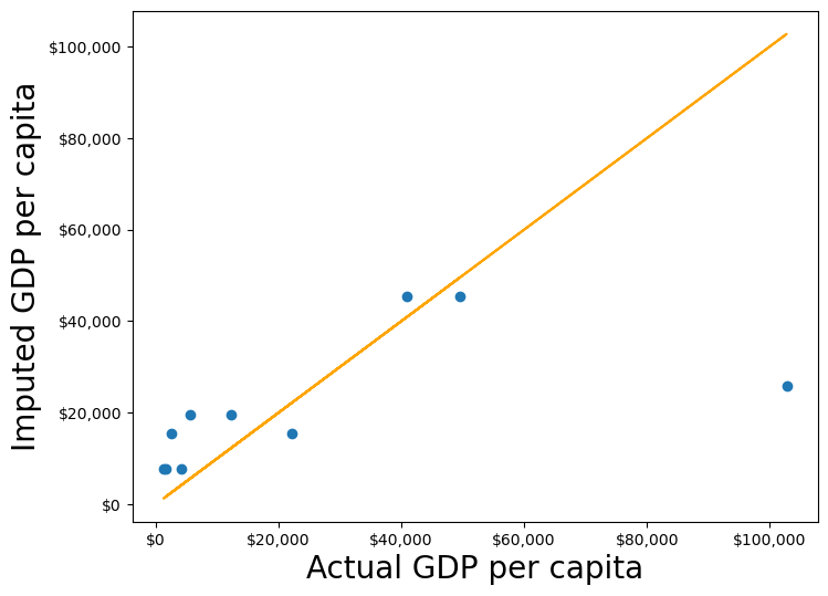

Approach 2: Using the groupby() and transform() methods.

The transform() function is a powerful tool for filling missing values in grouped data. It allows us to apply a function across each group and align the result back to the original DataFrame, making it perfect for filling missing values based on group statistics.

In this example, we use transform() to impute missing values in the gdpPerCapita column by filling them with the mean gdpPerCapita of each continent:

#Creating a copy of missing data to impute missing values
gdp_imputed_data = gdp_missing_data.copy()

#Grouping data by continent
grouped = gdp_missing_data.groupby('continent')

#Imputing missing values with the mean GDP per capita of the continent
gdp_imputed_data['gdpPerCapita'] = grouped['gdpPerCapita'].transform(lambda x: x.fillna(x.mean()))

plot_actual_vs_predicted()

RMSE= 25473.20645170116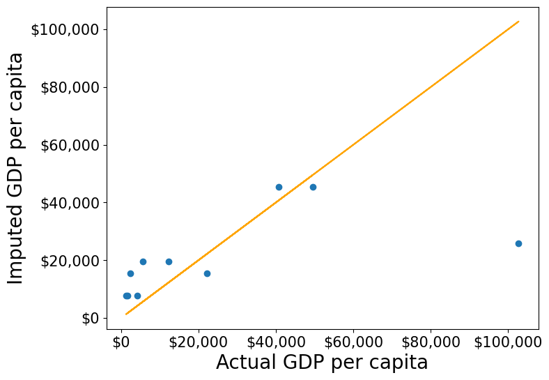

Using the transform() function, missing values in gdpPerCapita for each group are filled with the group’s mean gdpPerCapita. This approach is not only more convenient to write but also faster compared to using for loops. While a for loop imputes missing values one group at a time, transform() performs built-in operations (like mean, sum, etc.) in a way that is optimized internally, making it more efficient.

Let’s use apply() instead of transform() with groupby()

#Creating a copy of missing data to impute missing values
gdp_imputed_data = gdp_missing_data.copy()

#Grouping data by continent
grouped = gdp_missing_data.groupby('continent')

#Applying the lambda function on the 'gdpPerCapita' column of the groups
gdp_imputed_data['gdpPerCapita'] = grouped['gdpPerCapita'].apply(lambda x: x.fillna(x.mean()))

plot_actual_vs_predicted()

TypeError: incompatible index of inserted column with frame index

Why we ran into this error? and apply() doesn’t work?

Here’s a deeper look at why apply() doesn’t work as expected here:

12.4.2.1 Behavior of groupby().apply() vs. groupby().transform()

• groupby().apply(): This method applies a function to each group and returns the result with a hierarchical (multi-level) index by default. This hierarchical index can make it difficult to align the result back to a single column in the original DataFrame.

• groupby().transform(): In contrast, transform() is specifically designed to apply a function to each group and return a Series that is aligned with the original DataFrame’s index. This alignment makes it directly compatible for assignment to a new or existing column in the original DataFrame.

12.4.2.2 Why transform() Works for Imputation

When using transform() to fill missing values, it applies the function (e.g., fillna(x.mean())) based on each group’s statistics, such as the mean, while keeping the result aligned with the original DataFrame’s index. This allows for smooth assignment to a column in the DataFrame without any index mismatch issues.

Additionally, transform() applies the function to each element in a group independently and returns a result that has the same shape as the original data, making it ideal for adding or modifying columns.

12.4.3 Using filter() on Groups

The filter() function filters entire groups based on a condition. It evaluates each group and keeps only those that meet the specified criteria.

Example: Keep only the countries where the mean life expectancy is greater than 70

# keep only the continent where the mean life expectancy is greater than 74
gdp_lifeExp_data.groupby('continent').filter(lambda x: x['lifeExp'].mean() > 74)['continent'].unique()

array(['Oceania'], dtype=object)

# keep only the country where the mean life expectancy is greater than 74
gdp_lifeExp_data.groupby('country').filter(lambda x: x['lifeExp'].mean() > 74)['country'].unique()

array(['Australia', 'Canada', 'Denmark', 'France', 'Iceland', 'Italy',
       'Japan', 'Netherlands', 'Norway', 'Spain', 'Sweden', 'Switzerland'],
      dtype=object)

Using .nunique() get the number of countries that satisfy this condition

gdp_lifeExp_data.groupby('country').filter(lambda x: x['lifeExp'].mean() > 74)['country'].nunique()

12

12.5 Sampling data by group

If a dataset contains a large number of observations, operating on it can be computationally expensive. Instead, working on a sample of entire observations is a more efficient alterative. The groupby() method combined with apply() can be used for stratified random sampling from a large dataset.

Before taking the random sample, let us find the number of countries in each continent.

gdp_lifeExp_data.continent.value_counts()

continent
Africa      624
Asia        396
Europe      360
Americas    300
Oceania      24
Name: count, dtype: int64

Let us take a random sample of 650 observations from the entire dataset.

sample_lifeExp_data = gdp_lifeExp_data.sample(650)

Now, let us see the number of countries of each continent in our sample.

sample_lifeExp_data.continent.value_counts()

continent
Africa      241
Asia        149
Europe      142
Americas    109
Oceania       9
Name: count, dtype: int64

Some of the continent have a very low representation in the data. To rectify this, we can take a random sample of 130 observations from each of the 5 continents. In other words, we can take a random sample from each of the continent-based groups.

evenly_sampled_lifeExp_data = gdp_lifeExp_data.groupby('continent').apply(lambda x:x.sample(130, replace=True), include_groups=False)

group_sizes = evenly_sampled_lifeExp_data.groupby(level=0).size()
print(group_sizes)

continent
Africa      130
Americas    130
Asia        130
Europe      130
Oceania     130
dtype: int64

The above stratified random sample equally represents all the continent.

12.6 corr(): Correlation by group

The corr() method of the GroupBy object returns the correlation between all pairs of columns within each group.

Example: Find the correlation between lifeExp and gdpPercap for each continent-country level combination.

gdp_lifeExp_data.groupby(['continent','country']).apply(lambda x:x['lifeExp'].corr(x['gdpPercap']), include_groups=False)

continent  country       
Africa     Algeria           0.904471
           Angola           -0.301079
           Benin             0.843949
           Botswana          0.005597
           Burkina Faso      0.881677
                               ...   
Europe     Switzerland       0.980715
           Turkey            0.954455
           United Kingdom    0.989893
Oceania    Australia         0.986446
           New Zealand       0.974493
Length: 142, dtype: float64

Life expectancy is closely associated with GDP per capita across most continent-country combinations.

12.7 pivot_table()

The pivot_table() function in pandas is a powerful tool for performing groupwise aggregation in a structured format, similar to Excel’s pivot tables. It allows you to create a summary of data by grouping and aggregating it based on specified columns. Here’s an overview of how pivot_table() works for groupwise aggregation:

Note that pivot_table() is the same as pivot() except that pivot_table() aggregates the data as well in addition to re-arranging it.

Example: Consider the life expectancy dataset, calculate the average life expectancy for each country and year combination

pd.pivot_table(data = gdp_lifeExp_data, values = 'lifeExp',index = 'country', columns ='year',aggfunc = 'mean',margins = True)

year	1952	1957	1962	1967	1972	1977	1982	1987	1992	1997	2002	2007	All
country
Afghanistan	28.80100	30.332000	31.997000	34.02000	36.088000	38.438000	39.854000	40.822000	41.674000	41.763000	42.129000	43.828000	37.478833
Albania	55.23000	59.280000	64.820000	66.22000	67.690000	68.930000	70.420000	72.000000	71.581000	72.950000	75.651000	76.423000	68.432917
Algeria	43.07700	45.685000	48.303000	51.40700	54.518000	58.014000	61.368000	65.799000	67.744000	69.152000	70.994000	72.301000	59.030167
Angola	30.01500	31.999000	34.000000	35.98500	37.928000	39.483000	39.942000	39.906000	40.647000	40.963000	41.003000	42.731000	37.883500
Argentina	62.48500	64.399000	65.142000	65.63400	67.065000	68.481000	69.942000	70.774000	71.868000	73.275000	74.340000	75.320000	69.060417
...	...	...	...	...	...	...	...	...	...	...	...	...	...
West Bank and Gaza	43.16000	45.671000	48.127000	51.63100	56.532000	60.765000	64.406000	67.046000	69.718000	71.096000	72.370000	73.422000	60.328667
Yemen, Rep.	32.54800	33.970000	35.180000	36.98400	39.848000	44.175000	49.113000	52.922000	55.599000	58.020000	60.308000	62.698000	46.780417
Zambia	42.03800	44.077000	46.023000	47.76800	50.107000	51.386000	51.821000	50.821000	46.100000	40.238000	39.193000	42.384000	45.996333
Zimbabwe	48.45100	50.469000	52.358000	53.99500	55.635000	57.674000	60.363000	62.351000	60.377000	46.809000	39.989000	43.487000	52.663167
All	49.05762	51.507401	53.609249	55.67829	57.647386	59.570157	61.533197	63.212613	64.160338	65.014676	65.694923	67.007423	59.474439

143 rows × 13 columns

Explanation

• values: Specifies the column to aggregate (e.g., lifeExp in our example).
• index: Groups by the rows based on the country column.
• columns: Groups by the columns based on the year column.
• aggfunc: Uses mean to calculate the average life expectancy.

Common Aggregation Functions in pivot_table()

You can use various aggregation functions within pivot_table() to summarize data:

• mean – Calculates the average of values within each group.
• sum – Computes the total of values within each group.
• count – Counts the number of non-null entries within each group.
• min and max – Finds the minimum and maximum values within each group.

We can also use custom GroupBy aggregate functions with pivot_table().

Example: Find the \(90^{th}\) percentile of life expectancy for each country and year combination

pd.pivot_table(data = gdp_lifeExp_data, values = 'lifeExp',index = 'country', columns ='year',aggfunc = lambda x:np.percentile(x,90))

year	1952	1957	1962	1967	1972	1977	1982	1987	1992	1997	2002	2007
country
Afghanistan	28.801	30.332	31.997	34.020	36.088	38.438	39.854	40.822	41.674	41.763	42.129	43.828
Albania	55.230	59.280	64.820	66.220	67.690	68.930	70.420	72.000	71.581	72.950	75.651	76.423
Algeria	43.077	45.685	48.303	51.407	54.518	58.014	61.368	65.799	67.744	69.152	70.994	72.301
Angola	30.015	31.999	34.000	35.985	37.928	39.483	39.942	39.906	40.647	40.963	41.003	42.731
Argentina	62.485	64.399	65.142	65.634	67.065	68.481	69.942	70.774	71.868	73.275	74.340	75.320
...	...	...	...	...	...	...	...	...	...	...	...	...
Vietnam	40.412	42.887	45.363	47.838	50.254	55.764	58.816	62.820	67.662	70.672	73.017	74.249
West Bank and Gaza	43.160	45.671	48.127	51.631	56.532	60.765	64.406	67.046	69.718	71.096	72.370	73.422
Yemen, Rep.	32.548	33.970	35.180	36.984	39.848	44.175	49.113	52.922	55.599	58.020	60.308	62.698
Zambia	42.038	44.077	46.023	47.768	50.107	51.386	51.821	50.821	46.100	40.238	39.193	42.384
Zimbabwe	48.451	50.469	52.358	53.995	55.635	57.674	60.363	62.351	60.377	46.809	39.989	43.487

142 rows × 12 columns

12.8 crosstab()

12.8.1 Basic Usage of crosstab()

The crosstab() method is a special case of a pivot table for computing group frequncies (or size of each group).

# create a basic crosstab to see counts of countries in each continent
pd.crosstab(gdp_lifeExp_data['continent'], columns='count')

col_0	count
continent
Africa	624
Americas	300
Asia	396
Europe	360
Oceania	24

Use the margins=True argument to add totals (row and column margins) to the table. The All row and column provide totals for each age group and gender category.

# create a crosstab to see counts of countries in each continent and year
pd.crosstab(gdp_lifeExp_data['continent'], gdp_lifeExp_data['year'], margins=True)

year	1952	1957	1962	1967	1972	1977	1982	1987	1992	1997	2002	2007	All
continent
Africa	52	52	52	52	52	52	52	52	52	52	52	52	624
Americas	25	25	25	25	25	25	25	25	25	25	25	25	300
Asia	33	33	33	33	33	33	33	33	33	33	33	33	396
Europe	30	30	30	30	30	30	30	30	30	30	30	30	360
Oceania	2	2	2	2	2	2	2	2	2	2	2	2	24
All	142	142	142	142	142	142	142	142	142	142	142	142	1704

This table shows the count of each year in each continent group, helping us understand the year distribution across different continent groups. We may often use it to check if the data is representative of all groups that are of interest to us.

12.8.2 Using crosstab() with Aggregation Functions

You can specify a values column and an aggregation function (aggfunc) to summarize numerical data for each combination of categorical variables.

Example: find the mean life expectancy for each continent and year

# find the mean life expectancy for each country in each continent and year
pd.crosstab(gdp_lifeExp_data['continent'], gdp_lifeExp_data['year'], values=gdp_lifeExp_data['lifeExp'], aggfunc='mean')

year	1952	1957	1962	1967	1972	1977	1982	1987	1992	1997	2002	2007
continent
Africa	39.135500	41.266346	43.319442	45.334538	47.450942	49.580423	51.592865	53.344788	53.629577	53.598269	53.325231	54.806038
Americas	53.279840	55.960280	58.398760	60.410920	62.394920	64.391560	66.228840	68.090720	69.568360	71.150480	72.422040	73.608120
Asia	46.314394	49.318544	51.563223	54.663640	57.319269	59.610556	62.617939	64.851182	66.537212	68.020515	69.233879	70.728485
Europe	64.408500	66.703067	68.539233	69.737600	70.775033	71.937767	72.806400	73.642167	74.440100	75.505167	76.700600	77.648600
Oceania	69.255000	70.295000	71.085000	71.310000	71.910000	72.855000	74.290000	75.320000	76.945000	78.190000	79.740000	80.719500

12.9 Independent Study

12.9.1 Practice exercise 1

Read the table consisting of GDP per capita of countries from the webpage: https://en.wikipedia.org/wiki/List_of_countries_by_GDP_(nominal)_per_capita .

To only read the relevant table, read the tables that contain the word ‘Country’.

Estimate the GDP per capita of each country as the average of the estimates of the three agencies - IMF, United Nations and World Bank.

We need to do a bit of data cleaning before we could directly use the groupby() function. Follow the steps below:

1. Drop the “Year” column
2. Drop the level 1 column name (innermost level column)
3. Apply the following function on all the columns of the “Estimate” to convert them to numeric: f = lambda x:pd.to_numeric(x,errors = 'coerce')
4. Set the Country/Territory column as the index
5. Convert all other columns into numeric and coerce errors using ‘errors=’coerce’`
6. Drop rows with NaN values
7. Find the average GDP per capital across the three agencies

dfs = pd.read_html('https://en.wikipedia.org/wiki/List_of_countries_by_GDP_(nominal)_per_capita', match = 'Country')
gdp_data  = dfs[0]
gdp_data.head()

	Country/Territory	IMF[4][5]		World Bank[6]		United Nations[7]
	Country/Territory	Estimate	Year	Estimate	Year	Estimate	Year
0	Monaco	—	—	240862	2022	240535	2022
1	Liechtenstein	—	—	187267	2022	197268	2022
2	Luxembourg	135321	2024	128259	2023	125897	2022
3	Bermuda	—	—	123091	2022	117568	2022
4	Switzerland	106098	2024	99995	2023	93636	2022

# Flatten the MultiIndex to access column names
gdp_data.columns = [' '.join(col).strip() if isinstance(col, tuple) else col for col in gdp_data.columns]

# Drop all columns containing "Year"
gdp_data = gdp_data.loc[:, ~gdp_data.columns.str.contains('Year', case=False)]

gdp_data = gdp_data.rename(columns={"Country/Territory Country/Territory": "Country/Territory"})

gdp_data.head()

	Country/Territory	IMF	World Bank	United Nations
0	Monaco	—	240862	240535
1	Liechtenstein	—	187267	197268
2	Luxembourg	135321	128259	125897
3	Bermuda	—	123091	117568
4	Switzerland	106098	99995	93636

import re
column_name_cleaner = lambda x:re.split(r'\[', x)[0]

gdp_data.columns = gdp_data.columns.map(column_name_cleaner)
gdp_data.head()

	Country/Territory	IMF	World Bank	United Nations
0	Monaco	—	240862	240535
1	Liechtenstein	—	187267	197268
2	Luxembourg	135321	128259	125897
3	Bermuda	—	123091	117568
4	Switzerland	106098	99995	93636

# set the country column as the index
gdp_data.set_index('Country/Territory', inplace=True)

# convert all other columns into numeric and coerce errors
gdp_data = gdp_data.apply(pd.to_numeric, errors='coerce')

# drop rows with NaN values
gdp_data.dropna(inplace=True)

#find the average GDP per capita
gdp_data['Average GDP per capita'] = gdp_data.mean(axis=1)
gdp_data.head()

	IMF	World Bank	United Nations	Average GDP per capita
Country/Territory
Luxembourg	135321.0	128259.0	125897.0	129825.666667
Switzerland	106098.0	99995.0	93636.0	99909.666667
Ireland	103500.0	103685.0	105993.0	104392.666667
Norway	90434.0	87962.0	106623.0	95006.333333
Singapore	89370.0	84734.0	78115.0	84073.000000

12.9.2 Practice exercise 2

Read the spotify dataset from spotify_data.csv that contains information about tracks and artists

12.9.2.1

Find the mean and standard deviation of the track popularity for each genre.

12.9.2.2

Create a new categorical column, energy_lvl, with two levels – ‘Low energy’ and ‘High energy’ – using equal-sized bins based on the track’s energy level. Then, calculate the mean, standard deviation, and 90th percentile of track popularity for each genre and energy level combination

12.9.2.3

Find the mean and standard deviation of track popularity and danceability for each genre and energy level. What insights you can gain from the generated table

12.9.2.4

For each genre and energy level, find the mean and standard deviation of the track popularity, and the minimum and maximum values of loudness.

12.9.2.5

Find the most popular artist from each genre.

12.9.2.6

Filter the first 4 columns of the spotify dataset. Drop duplicate observartions in the resulting dataset using the Pandas DataFrame method drop_duplicates(). Find the top 3 most popular artists for each genre.

12.9.2.7

The spotify dataset has more than 200k observations. It may be expensive to operate with so many observations. Take a random sample of 650 observations to analyze spotify data, such that all genres are equally represented.

12.9.2.8

Find the correlation between danceability and track popularity for each genre-energy level combination.

12.9.2.9

Find the mean of track popularity for each genre-energy lvl combination such that each row corresponds to a genre, and the energy levels correspond to columns.

Hints: using pivot_table()

12.9.2.10

Find the \(90^{th}\) percentile of track popularity for each genre-energy lvl combination such that each row corresponds to a genre, and the energy levels correspond to columns.

Hints: using pivot_table()

12.9.2.11

Find the number of observations in each group, where each groups corresponds to a distinct genre-energy lvl combination

12.9.2.12

Find the percentage of observations in each group of the above table.

12.9.2.13

What percentage of unique tracks are contributed by the top 5 artists of each genre?

Hint: Find the top 5 artists based on artist_popularity for each genre. Count the total number of unique tracks (track_name) contributed by these artists. Divide this number by the total number of unique tracks in the data. The nunique() function will be useful.