9 Introduction to Data Visualization
“One picture is worth a thousand words” - Fred R. Barnard
Visual perception offers the highest bandwidth channel, as we acquire much more information through visual perception than with all of the other channels combined, as billions of our neurons are dedicated to this task. Moreover, the processing of visual information is, at its first stages, a highly parallel process. Thus, it is generally easier for humans to comprehend information with plots, diagrams and pictures, rather than with text and numbers. This makes data visualizations a vital part of data science. Some of the key purposes of data visualization are:
- Data visualization is the first step towards exploratory data analysis (EDA), which reveals trends, patterns, insights, or even irregularities in data.
- Data visualization can help explain the workings of complex mathematical models.
- Data visualization are an elegant way to summarise the findings of a data analysis project.
- Data visualizations (especially interactive ones such as those on Tableau) may be the end-product of data analytics project, where the stakeholders make decisions based on the visualizations.
9.1 The Art of Visualization: Choosing the Right Plot Type
There are various types of plots available, and selecting the appropriate one is crucial for successful data visualization. The choice primarily depends on two factors: * The type of data you are working with, and * The role of visualization in your data analysis
9.1.1 Data Classification for Visualization
Data visualization is commonly used to plot data in a pandas DataFrame. The data can be classified into two categories:
Numeric Data: This type of data represents quantities and can take any value within a range. Common examples include age, height, temperature, etc.
Categorical Data: This type of data represents distinct categories or groups. It can be nominal (no inherent order, like colors or names) or ordinal (with a defined order, like ratings).
9.1.2 The Role of Visualization in Data Analysis
Data visualization is essential for effectively communicating insights derived from data analysis. By using various visualization techniques, we can uncover patterns, and understand relationships. Below, we discuss different types of data exploration and the relevant visualizations used for each.
9.1.2.1 Univariate Exploration
Purpose: Univariate exploration analyzes a single variable to understand its distribution, central tendency, and spread.
9.1.2.1.1 Common Visualizations:
- Histograms: Display the frequency distribution of a numeric variable, helping to identify the shape of the data (e.g., normal, skewed).
- Box Plots: Summarize key statistics of a variable, including median, quartiles, and potential outliers.
- Bar Plots: Show the count or proportion of categorical variables, revealing the frequency of each category.
- Line Plots: Used to display trends in numeric data over time, helping to visualize changes in a variable.
9.1.2.1.2 Insights Gained:
- Identify outliers and anomalies.
- Understand the range and distribution of values.
- Determine central tendency (mean, median, mode).
9.1.2.2 Bivariate Analysis
Purpose: Bivariate analysis examines the relationship between two variables, helping to understand how changes in one variable might affect another.
9.1.2.2.1 Common Visualizations:
- Scatter Plots: Illustrate the relationship between two numeric variables, highlighting trends and correlations.
- Grouped Bar Plots: Compare categorical variables against a numeric variable, revealing trends across categories.
- Heatmaps: Represent correlation coefficients between pairs of variables, allowing easy identification of strong correlations.
9.1.2.2.2 Insights Gained:
- Assess the strength and direction of relationships (positive, negative, or no correlation).
- Identify potential predictive relationships for further analysis.
- Discover patterns that may indicate causal relationships.
9.1.2.3 Multivariate Analysis
Purpose: Multivariate analysis investigates more than two variables simultaneously, providing a comprehensive view of complex relationships and interactions.
9.1.2.3.1 Common Visualizations:
- Pair Plots: Show pairwise relationships in a dataset, facilitating quick insights into correlations among multiple variables.
- 3D Scatter Plots: Visualize the interaction between three numeric variables in a three-dimensional space.
- Facet Grids: Display multiple plots for different subsets of data, enabling comparisons across categories.
9.1.2.3.2 Insights Gained:
- Understand interactions and dependencies among multiple variables.
- Identify clusters or groups within the data.
- Enhance predictive modeling by considering multiple influences.
9.1.3 Summary
Choosing the appropriate plot depends on the data type and the specific analysis purpose. Numeric data typically requires plots that can handle continuous data (like line plots or histograms), while categorical data often benefits from comparisons (like bar plots or pie charts). Always consider what story you want to tell with your data and select your visualization method accordingly.
9.2 Visulization Tools
We’ll use three libraries for making data visualizations - pandas, matplotlib, and seaborn.
To get started, let’s import these libraries.
import pandas as pd
import matplotlib.pyplot as plt
import seaborn as sns

# let's import numpy as well
import numpy as np
9.2.1 Basic Plotting with Pandas
In previous chapters, we focused on using the pandas library for data reading and analysis. In addition to its powerful data manipulation capabilities, pandas also provides tools for creating basic plots, making it especially valuable for exploratory data analysis.
In this section, we will use the COVID dataset to demonstrate basic plotting techniques with pandas.
covid_df = pd.read_csv('./Datasets/covid.csv')
covid_df.head(5)| date | new_cases | total_cases | new_deaths | total_deaths | new_tests | total_tests | cases_per_million | deaths_per_million | tests_per_million | |
|---|---|---|---|---|---|---|---|---|---|---|
| 0 | 2019-12-31 | 0.0 | 0.0 | 0.0 | 0.0 | NaN | NaN | 0.0 | 0.0 | NaN |
| 1 | 2020-01-01 | 0.0 | 0.0 | 0.0 | 0.0 | NaN | NaN | 0.0 | 0.0 | NaN |
| 2 | 2020-01-02 | 0.0 | 0.0 | 0.0 | 0.0 | NaN | NaN | 0.0 | 0.0 | NaN |
| 3 | 2020-01-03 | 0.0 | 0.0 | 0.0 | 0.0 | NaN | NaN | 0.0 | 0.0 | NaN |
| 4 | 2020-01-04 | 0.0 | 0.0 | 0.0 | 0.0 | NaN | NaN | 0.0 | 0.0 | NaN |
Let’s begin by visualizing the trend of new COVID cases over time using a line plot.
A line plot is ideal for showing changes over continuous data, such as the progression of new cases over a series of dates.
covid_df.new_cases.plot()<Axes: >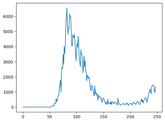
While this plot shows the overall trend, it’s hard to tell where the peak occurred, as there are no dates on the X-axis. We can use the date column as the index for the data frame to address this issue since it is a time series dataset
covid_df.set_index('date', inplace=True)covid_df.new_cases.plot(rot=45)<Axes: xlabel='date'>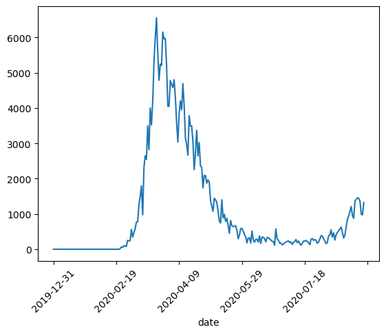
With the date set as the index, we can observe that the peak occurred around March 2020. Next, let’s plot both new cases and new deaths together to compare their trends over the same time period.
covid_df[['new_deaths', 'new_cases']].plot()<Axes: xlabel='date'>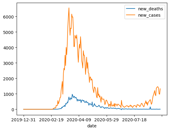
By default, pandas generates line plots when using the .plot method. However, there are several parameters you can adjust to enhance the appearance of the line plot.
covid_df[['new_deaths', 'new_cases']].plot(figsize=(12, 6), linewidth=2, marker='o')<Axes: xlabel='date'>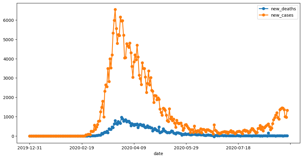
You can create other types of visualizations by setting the kind parameter in the plot function. The kind parameter accepts eleven different string values, which specify the type of plot:
- “area” is for area plots.
- “bar” is for vertical bar charts.
- “barh” is for horizontal bar charts.
- “box” is for box plots.
- “hexbin” is for hexbin plots.
- “hist” is for histograms.
- “kde” is for kernel density estimate charts.
- “density” is an alias for “kde”.
- “line” is for line graphs.
- “pie” is for pie charts.
- “scatter” is for scatter plots.
Let’s next create a scatter plot to visualize the relationship between new cases and new deaths, and explore whether there’s a correlation between them.
covid_df.plot(kind='scatter', x='new_cases', y='new_deaths', color='r', alpha=0.5);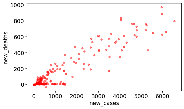
Next, let’s examine the distribution of new deaths using a histogram.
covid_df.new_deaths.plot(kind='hist', color='r', alpha=0.5, bins=50);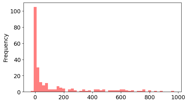
covid_df.new_cases.plot(kind='box');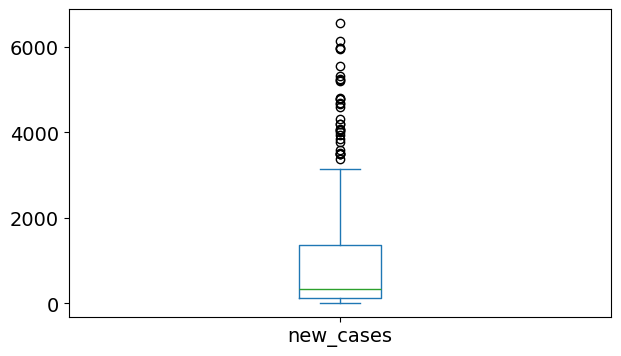
For more plot types and detailed information, refer to the official pandas documentation:
9.2.1.1 Limitation of using pandas for plotting
While pandas provides a straightforward way to create plots, there are some limitations to be aware of:
Customization: Pandas offers basic customization options, but it may not provide the level of detail or flexibility that you can achieve with matplotlib directly. For complex visualizations, you might need to switch to matplotlib for more control.
Plot Types: The range of plot types available in pandas is limited compared to what you can create with matplotlib or seaborn. For instance, advanced plots like violin plots or 3D plots require switching to other libraries.
Aesthetic Choices: The default aesthetics in pandas may not be as visually appealing as those created using seaborn or other specialized visualization libraries. For polished presentations, additional customization might be necessary.
9.2.2 Data Plotting with Matplotlib Pyplot Interface
Pandas data visualization is built on top of matplotlib. When you use the .plot() method in pandas, it internally calls matplotlib functions to create the plots.
Matplotlib is:
- a low-level graph plotting library in python that strives to emulate MATLAB,
- can be used in Python scripts, Python and IPython shells, Jupyter notebooks and web application servers.
- is mostly written in python, a few segments are written in C, Objective-C and Javascript for Platform compatibility.
9.2.2.1 Matplotlib pyplot
- Matplotlib is the whole package; pyplot is a module in matplotlib
- Most of the Matplotlib utilities lies under the pyplot module, and are usually imported under the plt alias:
import matplotlib.pyplot as plt9.2.2.2 Data Source
- Python lists, NumPy arrays as well as a pandas series
- However, all the sequences are internally converted to numpy arrays.
Let’s create a python list to illustrate basic plotting with Matplotlib pyplot
yield_apples = [0.895, 0.91, 0.919, 0.926, 0.929, 0.931]9.2.2.3 Basic Plotting
9.2.2.3.1 Plotting the overall trend
plt.plot(yield_apples)
Calling the plt.plot function draws the line chart as expected. It also returns a list of plots drawn [<matplotlib.lines.Line2D at 0x2194b571df0>], shown within the output. We can include a semicolon (;) at the end of the last statement in the cell to avoiding showing the output and display just the graph.
plt.plot(yield_apples);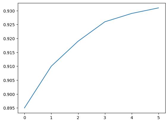
9.2.2.3.2 Customizing the X-axis
The X-axis of the plot currently shows list element indexes 0 to 5. The plot would be more informative if we could display the year for which we’re plotting the data. We can do this by two arguments plt.plot.
years = [2010, 2011, 2012, 2013, 2014, 2015]
yield_apples = [0.895, 0.91, 0.919, 0.926, 0.929, 0.931]
plt.plot(years, yield_apples);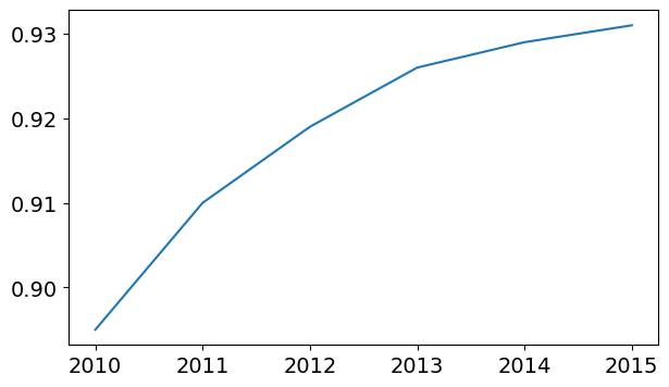
9.2.2.3.3 Ploting multiple lines
You can invoke the plt.plot function once for each line to plot multiple lines in the same graph. Let’s compare the yields of apples vs. oranges.
years = range(2000, 2012)
apples = [0.895, 0.91, 0.919, 0.926, 0.929, 0.931, 0.934, 0.936, 0.937, 0.9375, 0.9372, 0.939]
oranges = [0.962, 0.941, 0.930, 0.923, 0.918, 0.908, 0.907, 0.904, 0.901, 0.898, 0.9, 0.896, ]
plt.plot(years, apples)
plt.plot(years, oranges);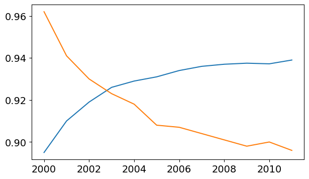
When plt.plot command is called without any formatting parameters, pyplot uses the following defaults:
- Figure size: 6.4 X 4.8 inches
- Plot style: solid line
- Linewidth: 1.5
- Color: Blue (code ‘b’, hex code: ‘#1f77b4’)
You can also edit default styles directly by modifying the matplotlib.rcParams dictionary. Learn more: https://matplotlib.org/3.2.1/tutorials/introductory/customizing.html#matplotlib-rcparams .
You can customize default plot styles by directly modifying the matplotlib.rcParams dictionary. For more details, visit the official Matplotlib guide on customizing with rcParams.
import matplotlib
matplotlib.rcParams['font.size'] = 14
matplotlib.rcParams['figure.figsize'] = (7, 4)
matplotlib.rcParams['figure.facecolor'] = '#00000000'
Conceptual model: Plotting in Matplotlib involves multiple levels of control, from setting the figure size to customizing individual text elements. To offer complete control over the plotting process, Matplotlib provides an object-oriented interface in a hierarchical structure. This approach allows users to create and manage Figure and Axes objects, which serve as the foundation for all plotting actions. In the next chapter, you will explore how to use this object-oriented interface to gain more precise control over your plots.
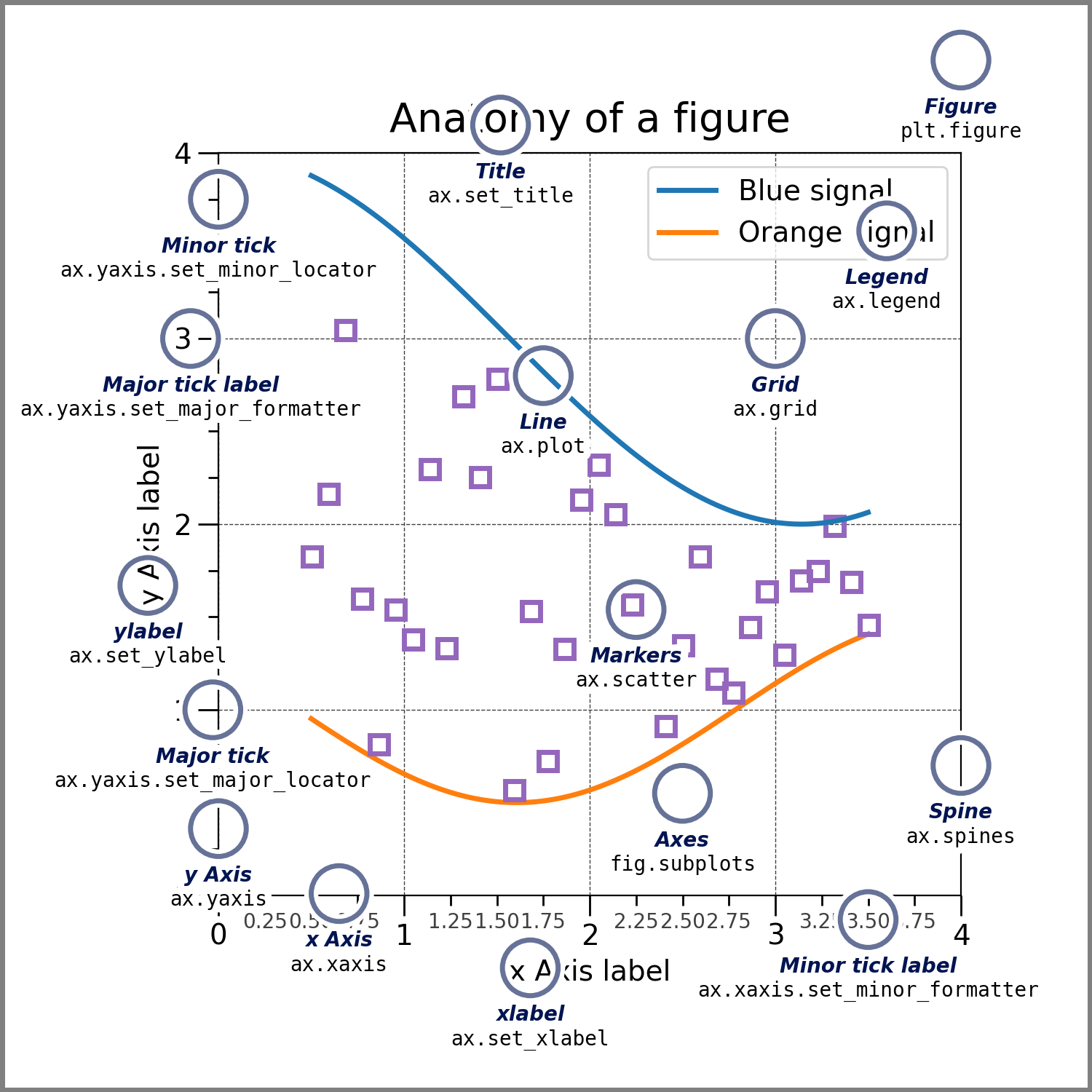
9.2.2.4 Enhancing the plot
Matplotlib provides a wide range of customizable components within a figure, allowing for fine-tuned control over every aspect of the plot. These components include elements like axes, labels, ticks, legends, and the overall layout. Each can be tailored to enhance the clarity, aesthetics, and effectiveness of the visual representation, making the plot more engaging and easier to interpret.
9.2.2.4.1 Adding Axis Lables
We can add labels to the axes to show what each axis represents using the plt.xlabel and plt.ylabel methods.
plt.plot(years, apples)
plt.plot(years, oranges)
plt.xlabel('Year')
plt.ylabel('Yield (tons per hectare)');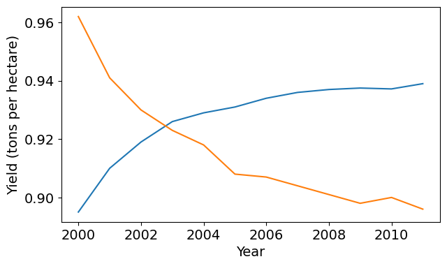
9.2.2.4.2 Adding Chart Title and Legend
To differentiate between multiple lines, we can include a legend within the graph using the plt.legend function. We can also set a title for the chart using the plt.title function.
plt.plot(years, apples)
plt.plot(years, oranges)

plt.xlabel('Year')
plt.ylabel('Yield (tons per hectare)')

plt.title("Crop Yields in Kanto")
plt.legend(['Apples', 'Oranges']);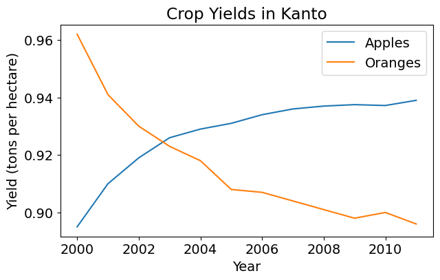
9.2.2.4.3 Adding Line Markers
We can also show markers for the data points on each line using the marker argument of plt.plot. Matplotlib provides many different markers, like a circle, cross, square, diamond, etc. You can find the full list of marker types here.
plt.plot(years, apples, marker='o')
plt.plot(years, oranges, marker='x')

plt.xlabel('Year')
plt.ylabel('Yield (tons per hectare)')

plt.title("Crop Yields in Kanto")
plt.legend(['Apples', 'Oranges']);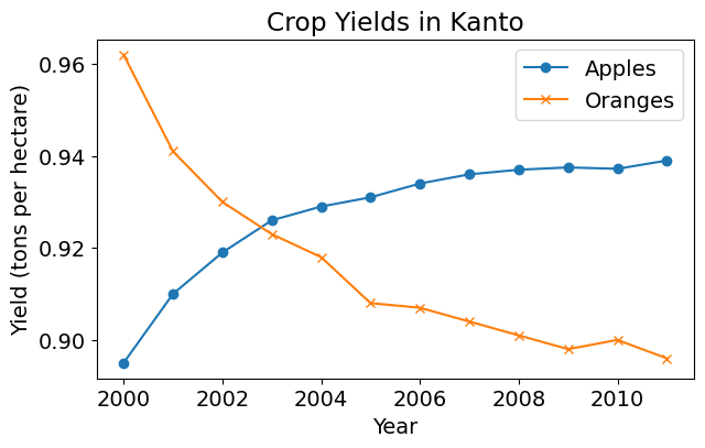
9.2.2.4.4 Styling Lines and Markers
The plt.plot function supports many arguments for styling lines and markers:
colororc: Set the color of the line (supported colors)linestyleorls: Choose between a solid or dashed linelinewidthorlw: Set the width of a linemarkersizeorms: Set the size of markersmarkeredgecolorormec: Set the edge color for markersmarkeredgewidthormew: Set the edge width for markersmarkerfacecolorormfc: Set the fill color for markersalpha: Opacity of the plot
Check out the documentation for plt.plot to learn more: https://matplotlib.org/api/_as_gen/matplotlib.pyplot.plot.html#matplotlib.pyplot.plot .
plt.plot(years, apples, marker='s', c='b', ls='-', lw=2, ms=8, mew=2, mec='navy')
plt.plot(years, oranges, marker='o', c='r', ls='--', lw=3, ms=10, alpha=.5)

plt.xlabel('Year')
plt.ylabel('Yield (tons per hectare)')

plt.title("Crop Yields in Kanto")
plt.legend(['Apples', 'Oranges']);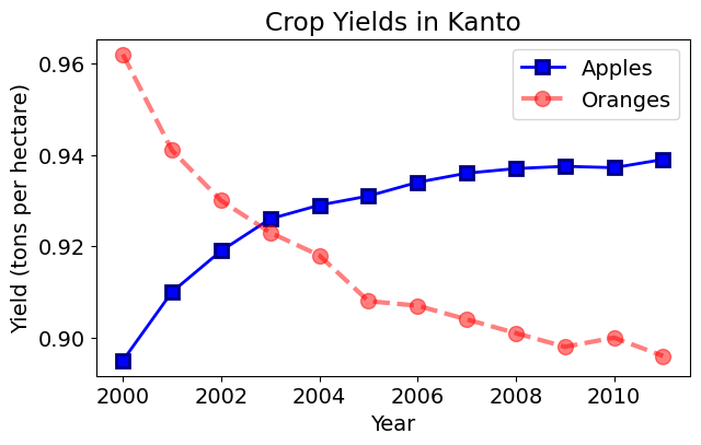
The fmt argument provides a shorthand for specifying the marker shape, line style, and line color. It can be provided as the third argument to plt.plot.
fmt = '[marker][line][color]'plt.plot(years, apples, 's-b')
plt.plot(years, oranges, 'o--r')
plt.xlabel('Year')
plt.ylabel('Yield (tons per hectare)')
plt.title("Crop Yields in Kanto")
plt.legend(['Apples', 'Oranges']);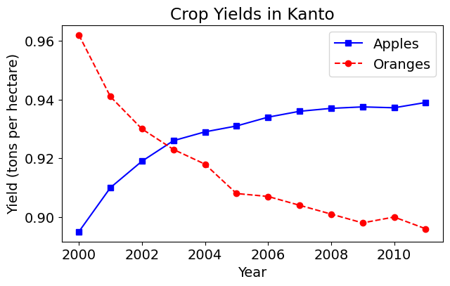
If you don’t specify a line style in fmt, only markers are drawn.
plt.plot(years, apples, 'sb')
plt.plot(years, oranges, 'or')
plt.title("Yield (tons per hectare)");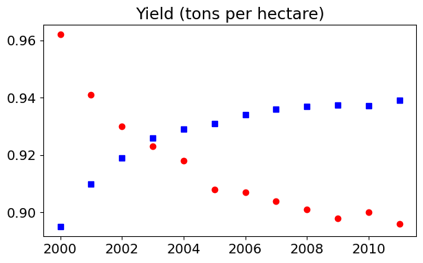
9.2.2.4.5 Changing the Figure Size
You can use the plt.figure function to change the size of the figure.
plt.figure(figsize=(6, 4))

plt.plot(years, oranges, 'or')
plt.title("Yield of Oranges (tons per hectare)");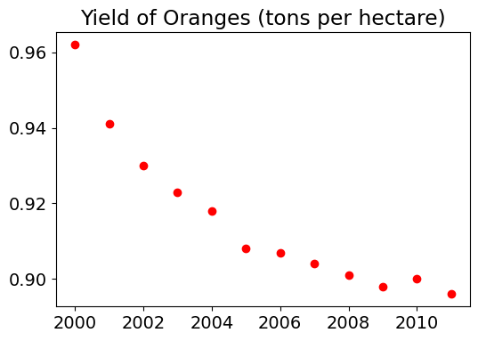
9.2.2.5 Plotting other types of plots with matplotlib pyplot
Let’s read the fifa_data.csv as our data source
fifa = pd.read_csv('./Datasets/fifa_data.csv')
fifa.head(5)| Unnamed: 0 | ID | Name | Age | Photo | Nationality | Flag | Overall | Potential | Club | ... | Composure | Marking | StandingTackle | SlidingTackle | GKDiving | GKHandling | GKKicking | GKPositioning | GKReflexes | Release Clause | |
|---|---|---|---|---|---|---|---|---|---|---|---|---|---|---|---|---|---|---|---|---|---|
| 0 | 0 | 158023 | L. Messi | 31 | https://cdn.sofifa.org/players/4/19/158023.png | Argentina | https://cdn.sofifa.org/flags/52.png | 94 | 94 | FC Barcelona | ... | 96.0 | 33.0 | 28.0 | 26.0 | 6.0 | 11.0 | 15.0 | 14.0 | 8.0 | €226.5M |
| 1 | 1 | 20801 | Cristiano Ronaldo | 33 | https://cdn.sofifa.org/players/4/19/20801.png | Portugal | https://cdn.sofifa.org/flags/38.png | 94 | 94 | Juventus | ... | 95.0 | 28.0 | 31.0 | 23.0 | 7.0 | 11.0 | 15.0 | 14.0 | 11.0 | €127.1M |
| 2 | 2 | 190871 | Neymar Jr | 26 | https://cdn.sofifa.org/players/4/19/190871.png | Brazil | https://cdn.sofifa.org/flags/54.png | 92 | 93 | Paris Saint-Germain | ... | 94.0 | 27.0 | 24.0 | 33.0 | 9.0 | 9.0 | 15.0 | 15.0 | 11.0 | €228.1M |
| 3 | 3 | 193080 | De Gea | 27 | https://cdn.sofifa.org/players/4/19/193080.png | Spain | https://cdn.sofifa.org/flags/45.png | 91 | 93 | Manchester United | ... | 68.0 | 15.0 | 21.0 | 13.0 | 90.0 | 85.0 | 87.0 | 88.0 | 94.0 | €138.6M |
| 4 | 4 | 192985 | K. De Bruyne | 27 | https://cdn.sofifa.org/players/4/19/192985.png | Belgium | https://cdn.sofifa.org/flags/7.png | 91 | 92 | Manchester City | ... | 88.0 | 68.0 | 58.0 | 51.0 | 15.0 | 13.0 | 5.0 | 10.0 | 13.0 | €196.4M |
5 rows × 89 columns
9.2.2.5.1 Histgram
plt.figure(figsize=(8,5))

plt.hist(fifa.Overall, color='#abcdef')

plt.ylabel('Number of Players')
plt.xlabel('Skill Level')
plt.title('Distribution of Player Skills in FIFA 2018')
Text(0.5, 1.0, 'Distribution of Player Skills in FIFA 2018')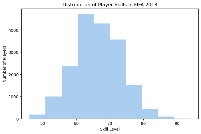
9.2.2.5.2 Bar chart
# plotting bar chart for the best players
plt.figure(figsize=(8,5))

foot_preference = fifa['Preferred Foot'].value_counts()

plt.bar(['Left', 'Right'], [foot_preference.iloc[1], foot_preference.iloc[0]], color='#abcdef')

plt.ylabel('Number of Players')
plt.title('Foot Preference of FIFA Players');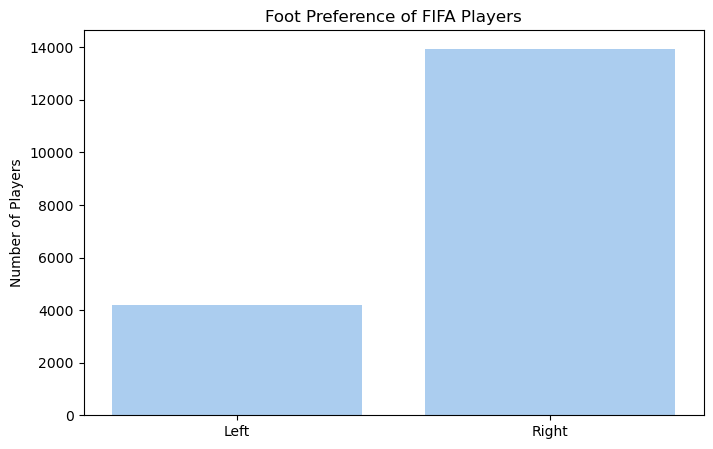
9.2.2.5.3 Pie chart
left = fifa.loc[fifa['Preferred Foot'] == 'Left'].count().iloc[0]
right = fifa.loc[fifa['Preferred Foot'] == 'Right'].count().iloc[0]

plt.figure(figsize=(8,5))

labels = ['Left', 'Right']
colors = ['#abcdef', '#aabbcc']

plt.pie([left, right], labels = labels, colors=colors, autopct='%.2f %%')

plt.title('Foot Preference of FIFA Players');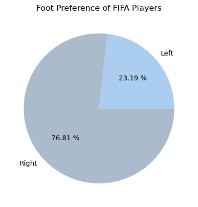
Another Pie Chart on wight of players
plt.figure(figsize=(8,5), dpi=100)

plt.style.use('ggplot')

fifa.Weight = [int(x.strip('lbs')) if type(x)==str else x for x in fifa.Weight]

light = fifa.loc[fifa.Weight < 125].count().iloc[0]
light_medium = fifa[(fifa.Weight >= 125) & (fifa.Weight < 150)].count().iloc[0]
medium = fifa[(fifa.Weight >= 150) & (fifa.Weight < 175)].count().iloc[0]
medium_heavy = fifa[(fifa.Weight >= 175) & (fifa.Weight < 200)].count().iloc[0]
heavy = fifa[fifa.Weight >= 200].count().iloc[0]

weights = [light,light_medium, medium, medium_heavy, heavy]
label = ['under 125', '125-150', '150-175', '175-200', 'over 200']
explode = (.4,.2,0,0,.4)

plt.title('Weight of Professional Soccer Players (lbs)')

plt.pie(weights, labels=label, explode=explode, pctdistance=0.8,autopct='%.2f %%');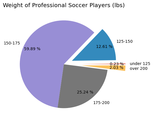
9.2.2.5.4 Box and Whiskers Chart
plt.figure(figsize=(5,8), dpi=100)

plt.style.use('default')

barcelona = fifa.loc[fifa.Club == "FC Barcelona"]['Overall']
madrid = fifa.loc[fifa.Club == "Real Madrid"]['Overall']
revs = fifa.loc[fifa.Club == "New England Revolution"]['Overall']

#bp = plt.boxplot([barcelona, madrid, revs], labels=['a','b','c'], boxprops=dict(facecolor='red'))
bp = plt.boxplot([barcelona, madrid, revs], tick_labels=['FC Barcelona','Real Madrid','NE Revolution'], patch_artist=True, medianprops={'linewidth': 2})

plt.title('Professional Soccer Team Comparison')
plt.ylabel('FIFA Overall Rating')

for box in bp['boxes']:
    # change outline color
    box.set(color='#4286f4', linewidth=2)
    # change fill color
    box.set(facecolor = '#e0e0e0' )
    # change hatch
    #box.set(hatch = '/')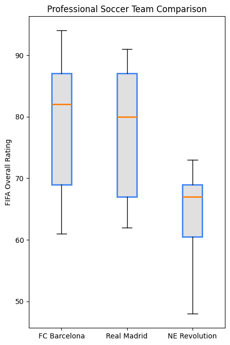
You’ve already learned how to create plots using Matplotlib’s Pyplot. Next, you’ll explore how to simplify and enhance your visualizations by using its powerful wrappers: Pandas and Seaborn.
9.2.2.6 Limitations of Using Matplotlib for Plotting
Matplotlib is a popular visualization library, but it has flaws.
- Defaults are not ideal (gridlines, background, etc need to be configured.)
- Library is low-level (doing anything complicated takes quite a bit of codes)
- Lack of integration with pandas data structures
To address these challenges, Seaborn act as higher-level interfaces to Matplotlib, offering better defaults, simpler syntax, and seamless integration with DataFrames.
9.2.3 Plotting with Seaborn
Seaborn is a powerful data visualization library built on top of Matplotlib, designed to make statistical plots easier and more attractive. It integrates seamlessly with Pandas, making it an excellent tool for plotting data from DataFrames. Seaborn comes with better default aesthetics and provides more specialized plots that are easy to implement.
Some of the key advantages of using Seaborn include:
- Simpler syntax: Seaborn simplifies the process of creating complex plots with just a few lines of code.
- Beautiful default styles: Seaborn’s default plots are more polished and aesthetically pleasing compared to Matplotlib’s defaults.
- Seamless Pandas integration: You can directly pass Pandas DataFrames to Seaborn, and it understands column names for axis labels and plot elements.
seaborn comes with 17 built-in datasets. That means you don’t have to spend a whole lot of your time finding the right dataset and cleaning it up to make Seaborn-ready; rather you will focus on the core features of Seaborn visualization techniques to solve problems.
import seaborn as sns
# get names of the builtin dataset
sns.get_dataset_names()
['anagrams',
'anscombe',
'attention',
'brain_networks',
'car_crashes',
'diamonds',
'dots',
'dowjones',
'exercise',
'flights',
'fmri',
'geyser',
'glue',
'healthexp',
'iris',
'mpg',
'penguins',
'planets',
'seaice',
'taxis',
'tips',
'titanic']9.2.3.1 Customizing Plot Aesthetics
Seaborn provides a convenient function called sns.set_style() that allows users to customize the visual appearance of their plots. This function is particularly useful for enhancing the aesthetics of visualizations, making them more appealing and easier to interpret.
9.2.3.1.1 Purpose of sns.set_style()
The primary purpose of sns.set_style() is to set the visual context and style for all plots created after the call. This allows for a consistent and visually pleasing representation of data across multiple visualizations.
9.2.3.1.2 Available Style Options
Seaborn offers several built-in styles that can be set using sns.set_style(). The options include:
darkgrid:- A dark background with a grid overlay.
- Ideal for visualizing data with many points or intricate details.
whitegrid:- A white background with a grid overlay.
- Provides a clean and professional look, suitable for most types of visualizations.
dark:- A dark background without gridlines.
- Useful for emphasizing data points without distractions from the grid.
white:- A simple white background without gridlines.
- Offers a minimalist aesthetic, focusing solely on the data.
ticks:- A white background with ticks on the axes.
- Combines the clarity of a white background with a bit of added detail for reference.
9.2.3.1.3 How to Use sns.set_style()
To apply a specific style, simply call sns.set_style() with the desired style name before creating your plots. Here’s an example:
sns.set_style("whitegrid")Let’s do a few common plots with Seaborn tips dataset
# Load data into a Pandas dataframe
flowers_df = sns.load_dataset("iris")
flowers_df.head()| sepal_length | sepal_width | petal_length | petal_width | species | |
|---|---|---|---|---|---|
| 0 | 5.1 | 3.5 | 1.4 | 0.2 | setosa |
| 1 | 4.9 | 3.0 | 1.4 | 0.2 | setosa |
| 2 | 4.7 | 3.2 | 1.3 | 0.2 | setosa |
| 3 | 4.6 | 3.1 | 1.5 | 0.2 | setosa |
| 4 | 5.0 | 3.6 | 1.4 | 0.2 | setosa |
9.2.3.2 Scatterplot
sns.scatterplot(x=flowers_df.sepal_length, y=flowers_df.sepal_width);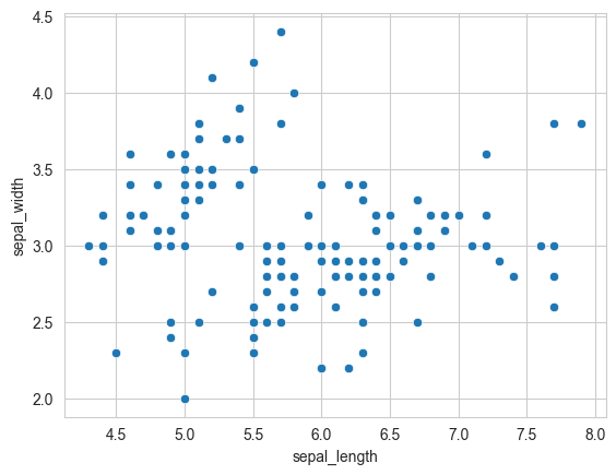
9.2.3.2.1 Adding Hues to the scatterplot
Notice how the points in the above plot seem to form distinct clusters with some outliers. We can color the dots using the flower species as a hue. We can also make the points larger using the s argument.
flowers_df.species.unique()array(['setosa', 'versicolor', 'virginica'], dtype=object)sns.scatterplot(x=flowers_df.sepal_length, y=flowers_df.sepal_width, hue=flowers_df.species, s=100);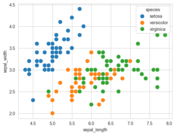
Adding hues makes the plot more informative. We can immediately tell that Setosa flowers have a smaller sepal length but higher sepal widths. In contrast, the opposite is true for Virginica flowers.
9.2.3.2.2 Customizing Seaborn Figures
Since Seaborn uses Matplotlib’s plotting functions internally, we can use functions like plt.figure and plt.title to modify the figure.
plt.figure(figsize=(12, 6))
plt.title('Sepal Dimensions')

sns.scatterplot(x=flowers_df.sepal_length,
                y=flowers_df.sepal_width,
                hue=flowers_df.species,
                s=100);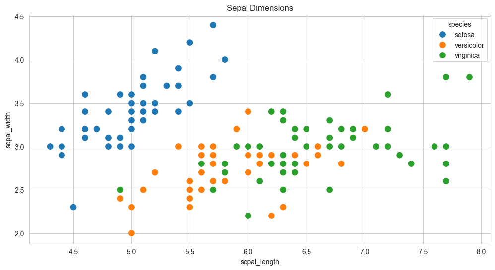
9.2.3.2.3 Integration with Pandas Data Frames
Seaborn has in-built support for Pandas data frames. Instead of passing each column as a series, you can provide column names and use the data argument to specify a data frame.
plt.title('Sepal Dimensions')
sns.scatterplot(x='sepal_length',
                y='sepal_width',
                hue='species',
                s=100,
                data=flowers_df);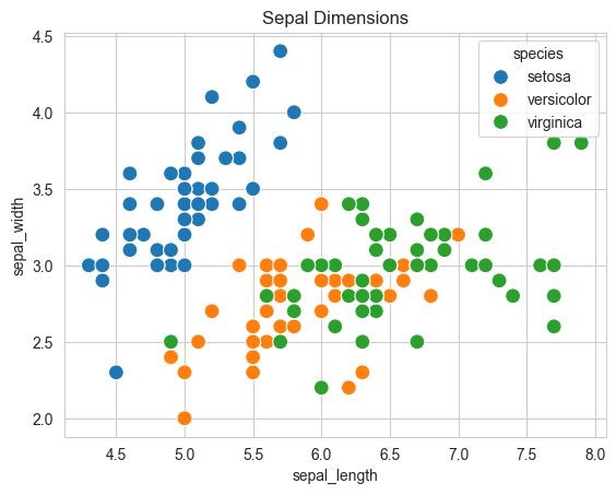
9.2.3.3 Histgram
sns.histplot(data=flowers_df, x='sepal_width');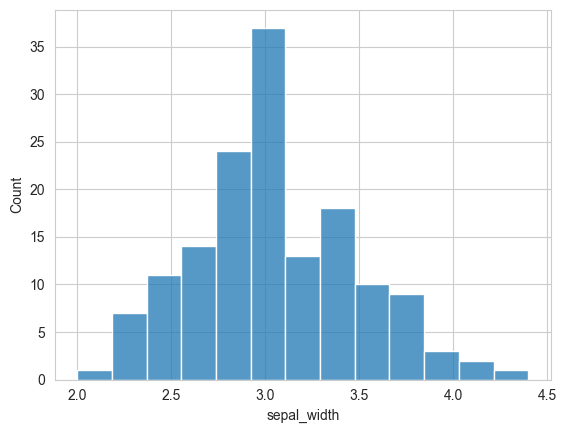
# show kde(kernal density estimate)
sns.histplot(data=flowers_df, x='sepal_width', kde=True);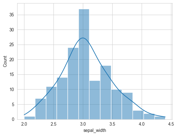
# adding hue
sns.histplot(data=flowers_df, x="sepal_width", hue="species");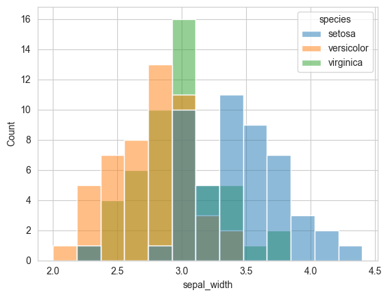
9.2.3.4 Barplot
tips_df = sns.load_dataset("tips")
sns.barplot(x='day', y='total_bill', data=tips_df);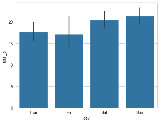
sns.barplot(x='day', y='tip', hue='sex', data=tips_df);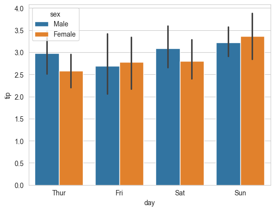
# make the bars horizontal simply by switching the axes
sns.barplot(x='tip', y='day', hue='sex', data=tips_df);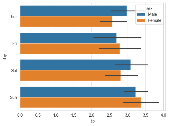
9.2.3.5 Boxplot
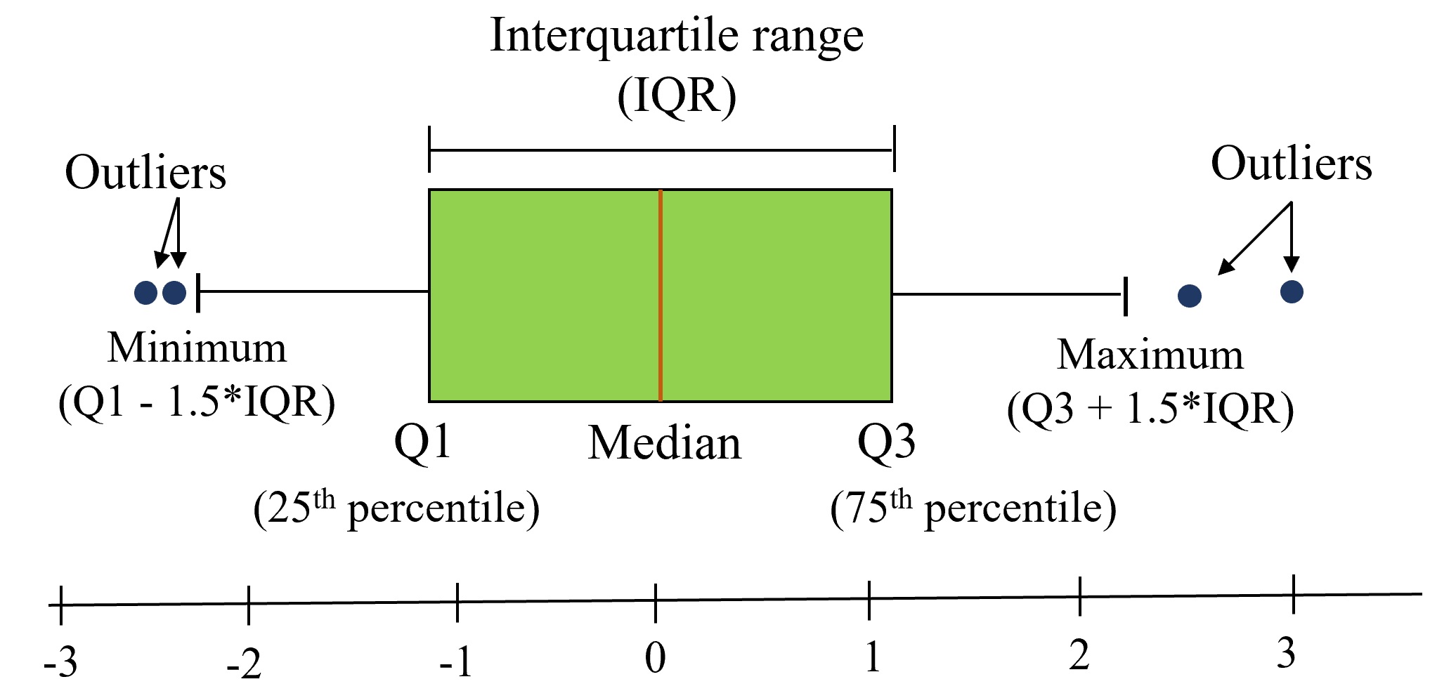
Purpose: Boxplots is a standardized way of visualizing the distribution of a continuous variable. They show five key metrics that describe the data distribution - median, 25th percentile value, 75th percentile value, minimum and maximum, as shown in the figure below. Note that the minimum and maximum exclude the outliers.
Example: Create a box plot to compare the distributions of total tips based on the day of the week, differentiating between male and female patrons.
sns.boxplot(data=tips_df, y='total_bill', x='day', hue='sex');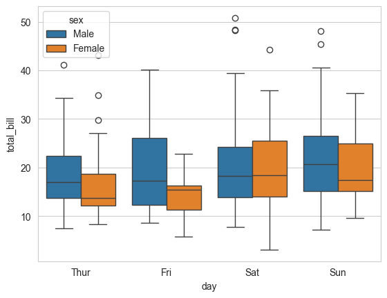
From the above plot, what you can observe?
9.2.3.6 Heatmap
Represent 2-dimensional data like a matrix or table using colors
flights_df = sns.load_dataset("flights").pivot(index="month", columns="year", values="passengers")
flights_df
# you will learn pivot in the later chapters| year | 1949 | 1950 | 1951 | 1952 | 1953 | 1954 | 1955 | 1956 | 1957 | 1958 | 1959 | 1960 |
|---|---|---|---|---|---|---|---|---|---|---|---|---|
| month | ||||||||||||
| Jan | 112 | 115 | 145 | 171 | 196 | 204 | 242 | 284 | 315 | 340 | 360 | 417 |
| Feb | 118 | 126 | 150 | 180 | 196 | 188 | 233 | 277 | 301 | 318 | 342 | 391 |
| Mar | 132 | 141 | 178 | 193 | 236 | 235 | 267 | 317 | 356 | 362 | 406 | 419 |
| Apr | 129 | 135 | 163 | 181 | 235 | 227 | 269 | 313 | 348 | 348 | 396 | 461 |
| May | 121 | 125 | 172 | 183 | 229 | 234 | 270 | 318 | 355 | 363 | 420 | 472 |
| Jun | 135 | 149 | 178 | 218 | 243 | 264 | 315 | 374 | 422 | 435 | 472 | 535 |
| Jul | 148 | 170 | 199 | 230 | 264 | 302 | 364 | 413 | 465 | 491 | 548 | 622 |
| Aug | 148 | 170 | 199 | 242 | 272 | 293 | 347 | 405 | 467 | 505 | 559 | 606 |
| Sep | 136 | 158 | 184 | 209 | 237 | 259 | 312 | 355 | 404 | 404 | 463 | 508 |
| Oct | 119 | 133 | 162 | 191 | 211 | 229 | 274 | 306 | 347 | 359 | 407 | 461 |
| Nov | 104 | 114 | 146 | 172 | 180 | 203 | 237 | 271 | 305 | 310 | 362 | 390 |
| Dec | 118 | 140 | 166 | 194 | 201 | 229 | 278 | 306 | 336 | 337 | 405 | 432 |
flights_df is a matrix with one row for each month and one column for each year. The values show the number of passengers (in thousands) that visited the airport in a specific month of a year. We can use the sns.heatmap function to visualize the footfall at the airport.
plt.title("No. of Passengers (1000s)")
sns.heatmap(flights_df);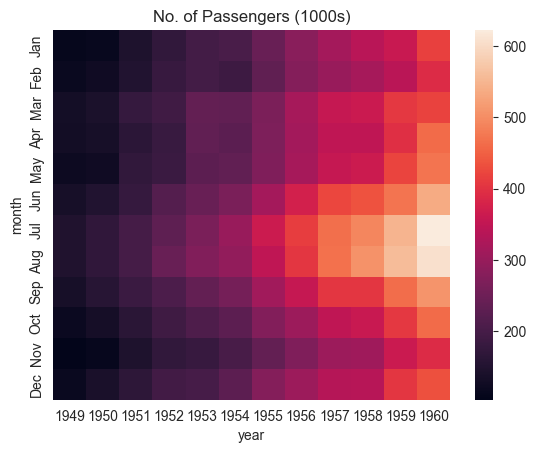
The brighter colors indicate a higher footfall at the airport. By looking at the graph, we can infer two things:
- The footfall at the airport in any given year tends to be the highest around July & August.
- The footfall at the airport in any given month tends to grow year by year.
We can also display the actual values in each block by specifying annot=True and using the cmap argument to change the color palette.
# fmt = "d" decimal integer. output are the number in base 10
plt.title("No. of Passengers (1000s)")
sns.heatmap(flights_df, fmt="d", annot=True, cmap='Blues');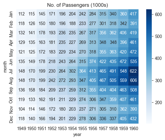
9.2.3.7 Correlation Map
A correlation map is a specific type of heatmap where the values represent the correlation coefficients between variables (ranging from -1 to 1). It visually shows the strength and direction of relationships between numerical variables.
Correlation may refer to any kind of association between two random variables. However, in this book, we will always consider correlation as the linear association between two random variables, or the Pearson’s correlation coefficient. Note that correlation does not imply causality and vice-versa.
The Pandas function corr() provides the pairwise correlation between all columns of a DataFrame, or between two Series. The function corrwith() provides the pairwise correlation of a DataFrame with another DataFrame or Series.
#Pairwise correlation amongst all columns
survey_data = pd.read_csv('./Datasets/survey_data_clean.csv')

survey_data.head()| Timestamp | fav_alcohol | parties_per_month | smoke | weed | introvert_extrovert | love_first_sight | learning_style | left_right_brained | personality_type | ... | used_python_before | dominant_hand | childhood_in_US | gender | region_of_residence | political_affliation | cant_change_math_ability | can_change_math_ability | math_is_genetic | much_effort_is_lack_of_talent | |
|---|---|---|---|---|---|---|---|---|---|---|---|---|---|---|---|---|---|---|---|---|---|
| 0 | 2022/09/13 1:43:34 pm GMT-5 | I don't drink | 1.0 | No | Occasionally | Introvert | 0 | Visual (learn best through images or graphic o... | Left-brained (logic, science, critical thinkin... | INFJ | ... | 1 | Right | 1 | Female | Northeast | Democrat | 0 | 1 | 0 | 0 |
| 1 | 2022/09/13 5:28:17 pm GMT-5 | Hard liquor/Mixed drink | 3.0 | No | Occasionally | Extrovert | 0 | Visual (learn best through images or graphic o... | Left-brained (logic, science, critical thinkin... | ESFJ | ... | 1 | Right | 1 | Male | West | Democrat | 0 | 1 | 0 | 0 |
| 2 | 2022/09/13 7:56:38 pm GMT-5 | Hard liquor/Mixed drink | 3.0 | No | Yes | Introvert | 0 | Kinesthetic (learn best through figuring out h... | Left-brained (logic, science, critical thinkin... | ISTJ | ... | 0 | Right | 0 | Female | International | No affiliation | 0 | 1 | 0 | 0 |
| 3 | 2022/09/13 10:34:37 pm GMT-5 | Hard liquor/Mixed drink | 12.0 | No | No | Extrovert | 0 | Visual (learn best through images or graphic o... | Left-brained (logic, science, critical thinkin... | ENFJ | ... | 0 | Right | 1 | Female | Southeast | Democrat | 0 | 1 | 0 | 0 |
| 4 | 2022/09/14 4:46:19 pm GMT-5 | I don't drink | 1.0 | No | No | Extrovert | 1 | Reading/Writing (learn best through words ofte... | Right-brained (creative, art, imaginative, int... | ENTJ | ... | 0 | Right | 1 | Female | Northeast | Democrat | 1 | 0 | 0 | 0 |
5 rows × 51 columns
#Pairwise correlation amongst all columns
survey_data.select_dtypes(include='number').corr()| parties_per_month | love_first_sight | num_insta_followers | expected_marriage_age | expected_starting_salary | minutes_ex_per_week | sleep_hours_per_day | farthest_distance_travelled | fav_number | internet_hours_per_day | ... | procrastinator | num_clubs | student_athlete | AP_stats | used_python_before | childhood_in_US | cant_change_math_ability | can_change_math_ability | math_is_genetic | much_effort_is_lack_of_talent | |
|---|---|---|---|---|---|---|---|---|---|---|---|---|---|---|---|---|---|---|---|---|---|
| parties_per_month | 1.000000 | 0.096129 | 0.239705 | -0.064079 | 0.114881 | 0.195561 | -0.052542 | -0.017081 | -0.050139 | 0.087390 | ... | -0.056871 | -0.010514 | 0.290830 | -0.013222 | -0.040033 | 0.081905 | -0.052912 | 0.055575 | -0.013374 | -0.029838 |
| love_first_sight | 0.096129 | 1.000000 | -0.024010 | -0.084406 | 0.080138 | 0.099244 | -0.025378 | -0.075539 | 0.105095 | -0.007652 | ... | 0.033951 | 0.083342 | 0.014595 | -0.062992 | -0.034692 | -0.118260 | 0.005254 | 0.020758 | -0.003710 | 0.013376 |
| num_insta_followers | 0.239705 | -0.024010 | 1.000000 | -0.130157 | 0.127226 | 0.099341 | -0.042421 | 0.011308 | -0.124763 | -0.028427 | ... | -0.089871 | 0.265958 | 0.044807 | 0.005947 | -0.016201 | 0.072622 | -0.150658 | 0.130774 | -0.018411 | -0.165899 |
| expected_marriage_age | -0.064079 | -0.084406 | -0.130157 | 1.000000 | -0.014881 | -0.088073 | 0.182009 | -0.024038 | -0.008924 | -0.029772 | ... | -0.020012 | -0.137069 | -0.036122 | 0.010447 | 0.052727 | 0.053759 | -0.072163 | 0.087633 | -0.086898 | 0.052813 |
| expected_starting_salary | 0.114881 | 0.080138 | 0.127226 | -0.014881 | 1.000000 | 0.134065 | -0.005078 | -0.028329 | -0.028125 | 0.017479 | ... | 0.054273 | -0.100922 | -0.026219 | -0.084894 | -0.094541 | 0.081142 | -0.011609 | 0.019171 | 0.078694 | 0.097265 |
| minutes_ex_per_week | 0.195561 | 0.099244 | 0.099341 | -0.088073 | 0.134065 | 1.000000 | 0.049593 | -0.153188 | 0.038758 | -0.028457 | ... | -0.045149 | -0.024572 | 0.576301 | -0.062544 | 0.057760 | 0.235492 | -0.101282 | 0.134430 | -0.047772 | -0.045141 |
| sleep_hours_per_day | -0.052542 | -0.025378 | -0.042421 | 0.182009 | -0.005078 | 0.049593 | 1.000000 | 0.104175 | -0.021909 | 0.017435 | ... | -0.176579 | -0.163860 | 0.058361 | -0.013909 | 0.096528 | -0.059468 | -0.058086 | 0.012174 | 0.027052 | -0.022025 |
| farthest_distance_travelled | -0.017081 | -0.075539 | 0.011308 | -0.024038 | -0.028329 | -0.153188 | 0.104175 | 1.000000 | -0.108661 | 0.049450 | ... | 0.032492 | -0.045214 | -0.158027 | 0.010580 | 0.012353 | -0.282821 | -0.046074 | 0.017935 | 0.110037 | 0.046895 |
| fav_number | -0.050139 | 0.105095 | -0.124763 | -0.008924 | -0.028125 | 0.038758 | -0.021909 | -0.108661 | 1.000000 | -0.013070 | ... | 0.085508 | -0.013696 | -0.014435 | 0.091011 | 0.030736 | 0.072894 | -0.032534 | 0.034319 | -0.063692 | -0.073777 |
| internet_hours_per_day | 0.087390 | -0.007652 | -0.028427 | -0.029772 | 0.017479 | -0.028457 | 0.017435 | 0.049450 | -0.013070 | 1.000000 | ... | 0.048239 | 0.064527 | -0.017944 | 0.001818 | 0.051970 | 0.033120 | -0.033902 | 0.050258 | 0.190205 | -0.053708 |
| only_child | -0.142519 | 0.124345 | -0.152184 | -0.043141 | -0.088648 | -0.123371 | 0.038126 | 0.214377 | -0.024419 | -0.035022 | ... | 0.073415 | -0.065484 | 0.064136 | 0.048031 | -0.139898 | -0.387711 | 0.023089 | -0.019982 | 0.058226 | 0.092372 |
| num_majors_minors | -0.073127 | 0.108730 | 0.050431 | -0.055280 | 0.021278 | 0.044450 | -0.024339 | -0.012779 | 0.023903 | -0.073775 | ... | -0.073806 | 0.311266 | -0.035500 | -0.068640 | -0.073388 | -0.153529 | -0.077501 | 0.024734 | -0.125809 | -0.064939 |
| high_school_GPA | 0.295646 | 0.069288 | 0.147402 | 0.017052 | 0.053354 | -0.076471 | -0.036904 | -0.064116 | -0.023081 | -0.034485 | ... | 0.031561 | -0.020854 | 0.006332 | 0.066837 | 0.072777 | 0.005606 | -0.095025 | 0.093416 | -0.082620 | 0.001373 |
| NU_GPA | -0.080548 | -0.114041 | 0.004702 | 0.011925 | -0.048069 | -0.108177 | 0.143997 | 0.038238 | -0.307656 | -0.014531 | ... | -0.269552 | 0.016724 | -0.027378 | -0.026544 | -0.008536 | -0.028968 | 0.002094 | -0.137330 | 0.036731 | 0.047840 |
| age | -0.032771 | 0.142384 | -0.230698 | 0.060416 | -0.102632 | -0.040906 | -0.035890 | 0.018811 | 0.096818 | 0.017515 | ... | -0.005892 | -0.127760 | -0.038315 | -0.026959 | 0.009924 | -0.152784 | -0.005954 | 0.014759 | -0.009315 | -0.126370 |
| height | -0.005405 | 0.216072 | 0.009318 | 0.044577 | 0.151517 | 0.182090 | -0.010650 | -0.235067 | 0.041298 | -0.023174 | ... | 0.063263 | 0.212038 | 0.080953 | 0.022484 | 0.016110 | 0.160309 | -0.055641 | 0.101811 | -0.064383 | 0.028509 |
| height_father | 0.126741 | 0.029419 | 0.179684 | 0.026949 | 0.011450 | 0.156227 | 0.097593 | -0.118669 | -0.032717 | -0.047314 | ... | -0.111183 | 0.022701 | 0.155003 | -0.010982 | -0.006480 | 0.137934 | -0.019593 | 0.008157 | 0.010222 | 0.060439 |
| height_mother | 0.079121 | 0.082684 | 0.129716 | 0.075316 | 0.033947 | 0.114181 | -0.044089 | -0.134582 | -0.029568 | -0.091417 | ... | -0.078265 | 0.091390 | 0.053258 | -0.100647 | -0.021396 | 0.119292 | 0.027120 | 0.034961 | -0.035449 | 0.074492 |
| procrastinator | -0.056871 | 0.033951 | -0.089871 | -0.020012 | 0.054273 | -0.045149 | -0.176579 | 0.032492 | 0.085508 | 0.048239 | ... | 1.000000 | 0.078341 | 0.094363 | 0.003053 | -0.016254 | -0.090868 | 0.002462 | 0.084419 | -0.001738 | 0.081471 |
| num_clubs | -0.010514 | 0.083342 | 0.265958 | -0.137069 | -0.100922 | -0.024572 | -0.163860 | -0.045214 | -0.013696 | 0.064527 | ... | 0.078341 | 1.000000 | -0.084562 | 0.087438 | 0.115062 | -0.021044 | -0.136249 | 0.070002 | -0.090570 | -0.108851 |
| student_athlete | 0.290830 | 0.014595 | 0.044807 | -0.036122 | -0.026219 | 0.576301 | 0.058361 | -0.158027 | -0.014435 | -0.017944 | ... | 0.094363 | -0.084562 | 1.000000 | -0.040686 | -0.049288 | 0.082888 | -0.066667 | -0.022576 | -0.060523 | 0.121232 |
| AP_stats | -0.013222 | -0.062992 | 0.005947 | 0.010447 | -0.084894 | -0.062544 | -0.013909 | 0.010580 | 0.091011 | 0.001818 | ... | 0.003053 | 0.087438 | -0.040686 | 1.000000 | 0.089517 | 0.106584 | 0.081109 | 0.029743 | -0.048375 | -0.018043 |
| used_python_before | -0.040033 | -0.034692 | -0.016201 | 0.052727 | -0.094541 | 0.057760 | 0.096528 | 0.012353 | 0.030736 | 0.051970 | ... | -0.016254 | 0.115062 | -0.049288 | 0.089517 | 1.000000 | 0.041928 | -0.011217 | 0.156806 | 0.088566 | 0.023366 |
| childhood_in_US | 0.081905 | -0.118260 | 0.072622 | 0.053759 | 0.081142 | 0.235492 | -0.059468 | -0.282821 | 0.072894 | 0.033120 | ... | -0.090868 | -0.021044 | 0.082888 | 0.106584 | 0.041928 | 1.000000 | -0.008575 | 0.057185 | -0.178003 | -0.013098 |
| cant_change_math_ability | -0.052912 | 0.005254 | -0.150658 | -0.072163 | -0.011609 | -0.101282 | -0.058086 | -0.046074 | -0.032534 | -0.033902 | ... | 0.002462 | -0.136249 | -0.066667 | 0.081109 | -0.011217 | -0.008575 | 1.000000 | -0.672777 | 0.294544 | 0.101835 |
| can_change_math_ability | 0.055575 | 0.020758 | 0.130774 | 0.087633 | 0.019171 | 0.134430 | 0.012174 | 0.017935 | 0.034319 | 0.050258 | ... | 0.084419 | 0.070002 | -0.022576 | 0.029743 | 0.156806 | 0.057185 | -0.672777 | 1.000000 | -0.361546 | -0.131047 |
| math_is_genetic | -0.013374 | -0.003710 | -0.018411 | -0.086898 | 0.078694 | -0.047772 | 0.027052 | 0.110037 | -0.063692 | 0.190205 | ... | -0.001738 | -0.090570 | -0.060523 | -0.048375 | 0.088566 | -0.178003 | 0.294544 | -0.361546 | 1.000000 | 0.154083 |
| much_effort_is_lack_of_talent | -0.029838 | 0.013376 | -0.165899 | 0.052813 | 0.097265 | -0.045141 | -0.022025 | 0.046895 | -0.073777 | -0.053708 | ... | 0.081471 | -0.108851 | 0.121232 | -0.018043 | 0.023366 | -0.013098 | 0.101835 | -0.131047 | 0.154083 | 1.000000 |
28 rows × 28 columns
Q: Which feature is the most correlated with NU_GPA?
survey_data.select_dtypes(include='number').corrwith(survey_data.NU_GPA).sort_values(ascending = False)NU_GPA 1.000000
sleep_hours_per_day 0.143997
num_majors_minors 0.141988
only_child 0.106440
much_effort_is_lack_of_talent 0.047840
farthest_distance_travelled 0.038238
math_is_genetic 0.036731
num_clubs 0.016724
expected_marriage_age 0.011925
num_insta_followers 0.004702
cant_change_math_ability 0.002094
used_python_before -0.008536
internet_hours_per_day -0.014531
AP_stats -0.026544
student_athlete -0.027378
childhood_in_US -0.028968
high_school_GPA -0.030883
height_father -0.040120
expected_starting_salary -0.048069
age -0.052039
height_mother -0.079276
parties_per_month -0.080548
height -0.099082
minutes_ex_per_week -0.108177
love_first_sight -0.114041
can_change_math_ability -0.137330
procrastinator -0.269552
fav_number -0.307656
dtype: float64sns.set(rc={'figure.figsize':(12,10)})
sns.heatmap(survey_data.select_dtypes(include='number').corr());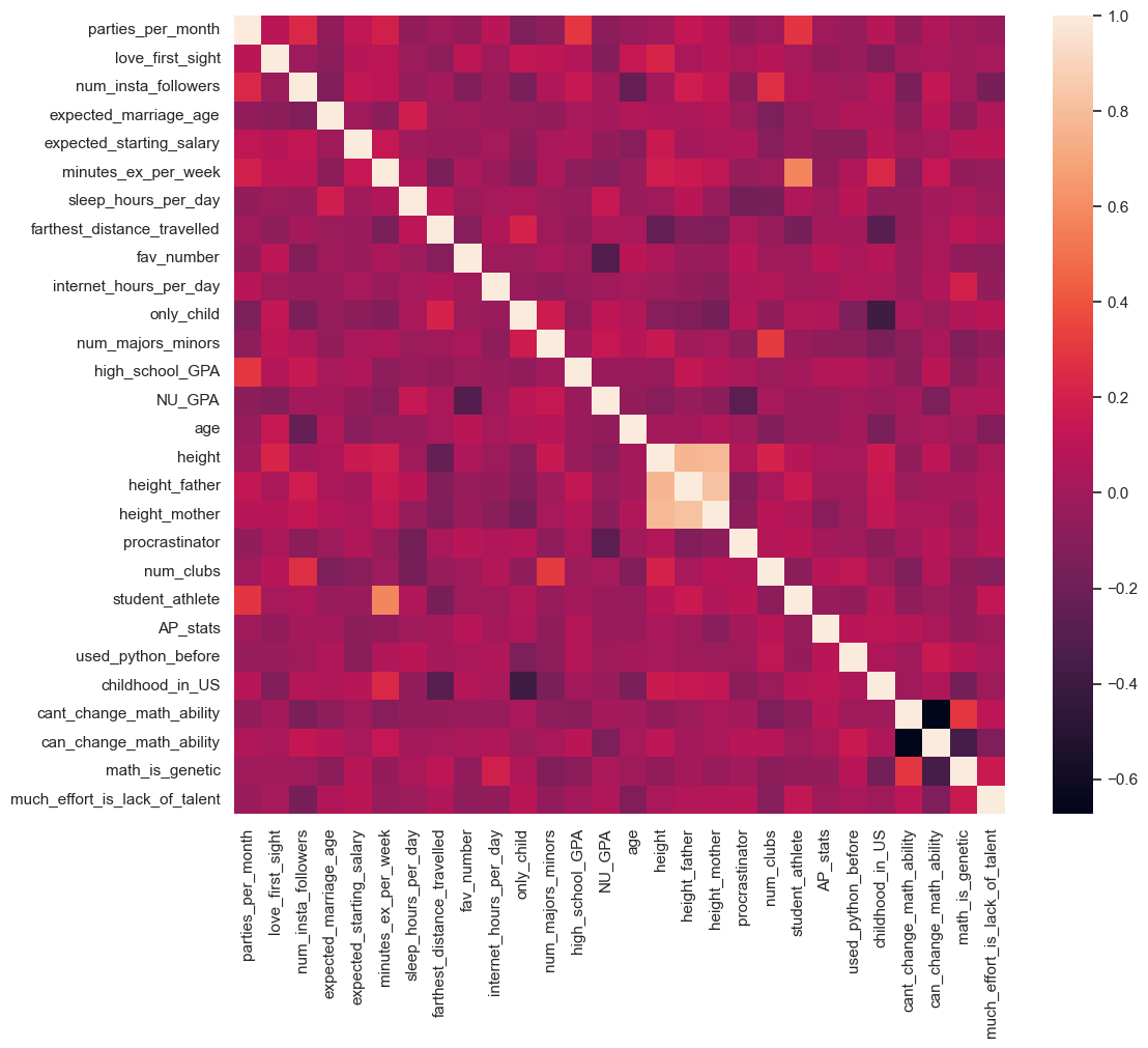
From the above map, we can see that:
student athleteis strongly postively correlated withminutes_ex_per_weekprocrastinatoris strongly negatively correlated withNU_GPA
9.3 Independent Study
9.3.1 Practice exercise 1
Read the gas_price.csv file and plot the trend for each country over the time using matplotlib pyplot
9.3.2 Practice exercise 2
9.3.2.1
Is NU_GPA associated with parties_per_month? Analyze the association separately for Sophomores, Juniors, and Seniors (categories of the variable school_year).
Make scatterplots of NU_GPA vs parties_per_month in a 1 x 3 grid, where each grid is for a distinct school_year. Plot the trendline as well for each scatterplot. Use the file survey_data_clean.csv.
9.3.2.2
Capping the the values of parties_per_month to 30, and make the visualizations again.
9.3.3 Practice exercise 3
How does the expected marriage age of the people of STAT303-1 depend on their characteristics? We’ll use visualizations to answer this question. Use data from the file survey_data_clean.csv. Proceed as follows:
9.3.3.1
Make a visualization that compares the mean expected_marriage_age of introverts and extroverts (use the variable introvert_extrovert). What insights do you obtain?
9.3.3.2
Does the mean expected_marriage_age of introverts and extroverts depend on whether they believe in love in first sight (variable name: love_first_sight)? Update the previous visualization to answer the question.
9.3.3.3
In addition to love_first_sight, does the mean expected_marriage_age of introverts and extroverts depend on whether they are a procrastinator (variable name: procrastinator)? Update the previous visualization to answer the question.
9.3.3.4
Is there any critical information missing in the above visualizations that, if revealed, may cast doubts on the patterns observed in them?
9.3.4 Practice exercise 4
Read Australia_weather.csv,
9.3.4.1
Create a histogram showing the distributions of maximum temperature in Sydney, Canberra and Melbourne.
9.3.4.2
Make a density plot showing the distributions of maximum temperature in Sydney, Canberra and Melbourne.
9.3.4.3
Show the distributions of the maximum and minimum temperatures in a single plot.
9.3.4.4
Create a scatter plot with a trendline for MinTemp and MaxTemp, including a confidence interval.
Hint: Using Seaborn, the regplot() function enables us to overlay a trendline on the scatter plot, complete with a 95% confidence interval for the trendline