13 Data Reshaping and Enrichment

In this chapter, we will explore how to reshape and enrich data using pandas. Data reshaping and enriching are essential steps in data preprocessing because they help transform raw data into a more structured, useful, and meaningful format that can be effectively used for analysis or modeling.

13.1 Data Reshaping

Data reshaping involves altering the structure of the data to suit the requirements of the analysis or modeling process. This is often needed when the data is in a format that is difficult to analyze or when it needs to be organized in a specific way.

13.1.1 Why Data Reshaping is Important:

Improves Data Organization: Raw data may be in a long format, where each observation is recorded on a separate row, or it may be in a wide format, where the same variable is spread across multiple columns. Reshaping allows you to reorganize the data into a format that is more suitable for analysis, such as turning multiple columns into a single column (melting) or aggregating rows into summary statistics (pivoting).
Facilitates Analysis: Some analysis techniques require specific data formats. For example, many machine learning algorithms require data in a matrix form, where each row represents a sample and each column represents a feature. Reshaping helps to convert data into this format.
Simplifies Visualization: Visualizing data is easier when it is in the right shape. For instance, plotting categorical data across time is easier when the data is in a tidy format, rather than having multiple variables spread across columns.
Efficient Grouping and Aggregation: In some cases, you may want to group data by certain categories or time periods, and reshaping can help aggregate data effectively for summarization.

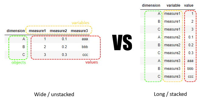
13.1.2 Wide vs. Long Data Format in Data Reshaping

Wide Format: Each variable in its own column; each row represents a unit, and data for multiple variables is spread across columns.
Long Format: Variables are stacked into one column per variable, with additional columns used to indicate time, categories, or other distinctions, leading to a greater number of rows.

To reshape between these two formats, you can use pandas functions such as pivot_table(), melt(), stack(), and unstack(). Let’s next take a look at each of these methods one by one.

Throughout this section, we will continue using the gdp_lifeExpectancy.csv dataset. Let’s start by reading the CSV file into a pandas DataFrame.

import pandas as pd
import numpy as np
import seaborn as sns
import matplotlib.pyplot as plt

%matplotlib inline

# Load the data
gdp_lifeExp_data = pd.read_csv('./Datasets/gdp_lifeExpectancy.csv')
gdp_lifeExp_data.head()

	country	continent	year	lifeExp	pop	gdpPercap
0	Afghanistan	Asia	1952	28.801	8425333	779.445314
1	Afghanistan	Asia	1957	30.332	9240934	820.853030
2	Afghanistan	Asia	1962	31.997	10267083	853.100710
3	Afghanistan	Asia	1967	34.020	11537966	836.197138
4	Afghanistan	Asia	1972	36.088	13079460	739.981106

13.1.3 Pivoting “long” to “wide” using `pivot_table()`

In the last chapter, we learned that pivot_table() is a powerful tool for performing groupwise aggregation in a structured format. The pivot_table() function is used to reshape data by specifying columns for the index, columns, and values.

13.1.3.1 Pivoting a single column

Consider the life expectancy dataset. Let’s calculate the average life expectancy for each combination of country and year.

gdp_lifeExp_data_pivot = gdp_lifeExp_data.pivot_table(index=['continent','country'], columns='year', values='lifeExp', aggfunc='mean')
gdp_lifeExp_data_pivot.head()

	year	1952	1957	1962	1967	1972	1977	1982	1987	1992	1997	2002	2007
continent	country
Africa	Algeria	43.077	45.685	48.303	51.407	54.518	58.014	61.368	65.799	67.744	69.152	70.994	72.301
	Angola	30.015	31.999	34.000	35.985	37.928	39.483	39.942	39.906	40.647	40.963	41.003	42.731
	Benin	38.223	40.358	42.618	44.885	47.014	49.190	50.904	52.337	53.919	54.777	54.406	56.728
	Botswana	47.622	49.618	51.520	53.298	56.024	59.319	61.484	63.622	62.745	52.556	46.634	50.728
	Burkina Faso	31.975	34.906	37.814	40.697	43.591	46.137	48.122	49.557	50.260	50.324	50.650	52.295

Explanation

values: Specifies the column to aggregate (e.g., lifeExp in our example).
index: Groups by the rows based on the continent and country column.
columns: Groups by the columns based on the year column.
aggfunc: Uses mean to calculate the average life expectancy.

With values of year as columns, it is easy to compare any metric for different years.

#visualizing the change in life expectancy of all countries in 2007 as compared to that in 1957, i.e., the overall change in life expectancy in 50 years. 
sns.scatterplot(data = gdp_lifeExp_data_pivot, x = 1957,y=2007,hue = 'continent')
sns.lineplot(data = gdp_lifeExp_data_pivot, x = 1957,y = 1957);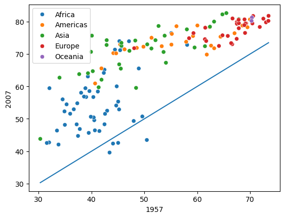

Observe that for some African countries, the life expectancy has decreased after 50 years. It is worth investigating these countries to identify factors associated with the decrease.

Another way to visualize a pivot table is by using a heatmap, which represents the 2D table as a matrix of colors, making it easier to interpret patterns and trends.

# Plotting a heatmap to visualize the life expectancy of all countries in all years, figure size is set to 15x10
plt.figure(figsize=(10,10))
plt.title("Life expectancy of all countries in all years")
sns.heatmap(gdp_lifeExp_data_pivot);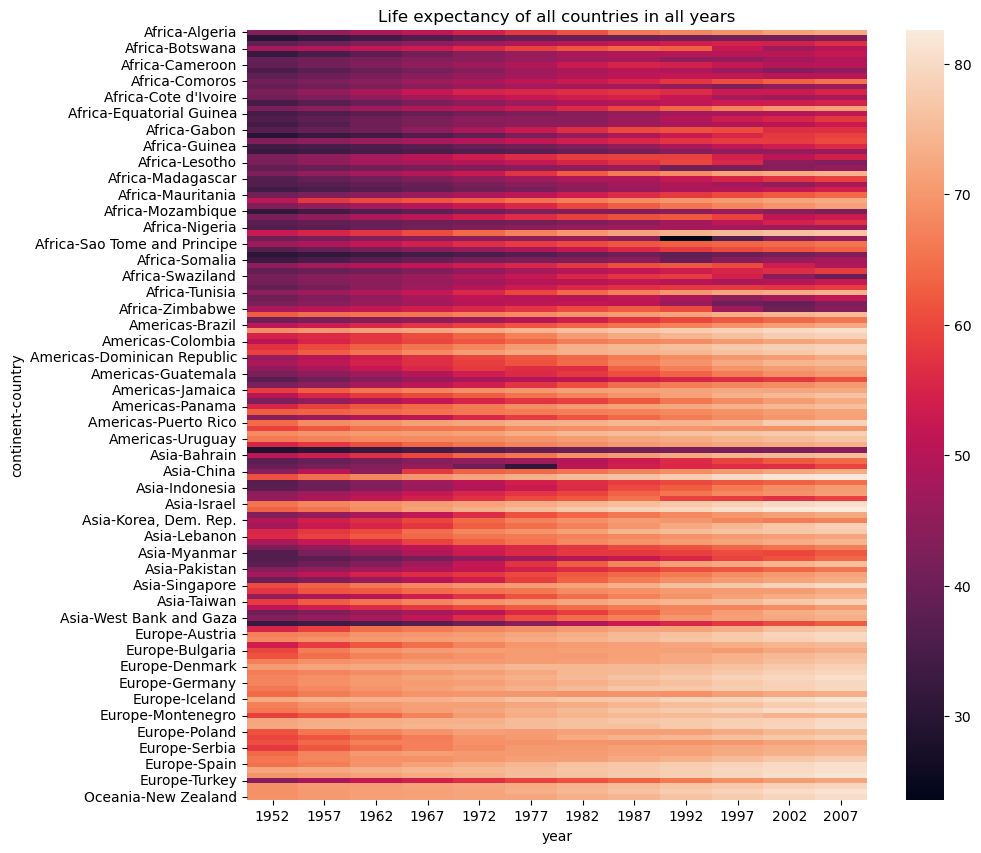

Common Aggregation Functions in pivot_table()

You can use various aggregation functions within pivot_table() to summarize data:

mean – Calculates the average of values within each group.
sum – Computes the total of values within each group.
count – Counts the number of non-null entries within each group.
min and max – Finds the minimum and maximum values within each group.

We can also define our own custom aggregation function and pass it to the aggfunc parameter of the pivot_table() function

For Example: Find the \(90^{th}\) percentile of life expectancy for each country and year combination

pd.pivot_table(data = gdp_lifeExp_data, values = 'lifeExp',index = 'country', columns ='year',aggfunc = lambda x:np.percentile(x,90))

year	1952	1957	1962	1967	1972	1977	1982	1987	1992	1997	2002	2007
country
Afghanistan	28.801	30.332	31.997	34.020	36.088	38.438	39.854	40.822	41.674	41.763	42.129	43.828
Albania	55.230	59.280	64.820	66.220	67.690	68.930	70.420	72.000	71.581	72.950	75.651	76.423
Algeria	43.077	45.685	48.303	51.407	54.518	58.014	61.368	65.799	67.744	69.152	70.994	72.301
Angola	30.015	31.999	34.000	35.985	37.928	39.483	39.942	39.906	40.647	40.963	41.003	42.731
Argentina	62.485	64.399	65.142	65.634	67.065	68.481	69.942	70.774	71.868	73.275	74.340	75.320
...	...	...	...	...	...	...	...	...	...	...	...	...
Vietnam	40.412	42.887	45.363	47.838	50.254	55.764	58.816	62.820	67.662	70.672	73.017	74.249
West Bank and Gaza	43.160	45.671	48.127	51.631	56.532	60.765	64.406	67.046	69.718	71.096	72.370	73.422
Yemen, Rep.	32.548	33.970	35.180	36.984	39.848	44.175	49.113	52.922	55.599	58.020	60.308	62.698
Zambia	42.038	44.077	46.023	47.768	50.107	51.386	51.821	50.821	46.100	40.238	39.193	42.384
Zimbabwe	48.451	50.469	52.358	53.995	55.635	57.674	60.363	62.351	60.377	46.809	39.989	43.487

142 rows × 12 columns

13.1.4 Melting “wide” to “long” using `melt()`

Melting is the inverse of pivoting. It transforms columns into rows. The melt() function is used when you want to unpivot a DataFrame, turning multiple columns into rows.

Let’s first consider gdp_lifeExp_data_pivot created in the previous section

gdp_lifeExp_data_pivot.head()

	year	1952	1957	1962	1967	1972	1977	1982	1987	1992	1997	2002	2007
continent	country
Africa	Algeria	43.077	45.685	48.303	51.407	54.518	58.014	61.368	65.799	67.744	69.152	70.994	72.301
	Angola	30.015	31.999	34.000	35.985	37.928	39.483	39.942	39.906	40.647	40.963	41.003	42.731
	Benin	38.223	40.358	42.618	44.885	47.014	49.190	50.904	52.337	53.919	54.777	54.406	56.728
	Botswana	47.622	49.618	51.520	53.298	56.024	59.319	61.484	63.622	62.745	52.556	46.634	50.728
	Burkina Faso	31.975	34.906	37.814	40.697	43.591	46.137	48.122	49.557	50.260	50.324	50.650	52.295

gdp_lifeExp_data_pivot.melt(value_name='lifeExp', var_name='year', ignore_index=False)

		year	lifeExp
continent	country
Africa	Algeria	1952	43.077
	Angola	1952	30.015
	Benin	1952	38.223
	Botswana	1952	47.622
	Burkina Faso	1952	31.975
...	...	...	...
Europe	Switzerland	2007	81.701
	Turkey	2007	71.777
	United Kingdom	2007	79.425
Oceania	Australia	2007	81.235
Oceania	New Zealand	2007	80.204

1704 rows × 2 columns

With the above DataFrame, we can visualize the mean life expectancy against year separately for each country in each continent.

13.1.5 Stacking and Unstacking using `stack()` and `unstack()`

Stacking and unstacking are powerful techniques used to reshape DataFrames by moving data between rows and columns. These operations are particularly useful when working with multi-level index or multi-level columns, where the data is structured in a hierarchical format.

stack(): Converts columns into rows, which means it “stacks” the data into a long format.
unstack(): Converts rows into columns, reversing the effect of stack().

Let’s use the GDP per capita dataset and create a DataFrame with a multi-level index (e.g., continent, country) and multi-level columns (e.g., lifeExp , gdpPercap, and pop).

# calculate the average and standard deviation of life expectancy, population, and GDP per capita for countries across the years.

gdp_lifeExp_multilevel_data = gdp_lifeExp_data.groupby(['continent', 'country'])[['lifeExp', 'pop', 'gdpPercap']].agg(['mean', 'std'])
gdp_lifeExp_multilevel_data

		lifeExp		pop		gdpPercap
		mean	std	mean	std	mean	std
continent	country
Africa	Algeria	59.030167	10.340069	1.987541e+07	8.613355e+06	4426.025973	1310.337656
	Angola	37.883500	4.005276	7.309390e+06	2.672281e+06	3607.100529	1165.900251
	Benin	48.779917	6.128681	4.017497e+06	2.105002e+06	1155.395107	159.741306
	Botswana	54.597500	5.929476	9.711862e+05	4.710965e+05	5031.503557	4178.136987
	Burkina Faso	44.694000	6.845792	7.548677e+06	3.247808e+06	843.990665	183.430087
...	...	...	...	...	...	...	...
Europe	Switzerland	75.565083	4.011572	6.384293e+06	8.582009e+05	27074.334405	6886.463308
	Turkey	59.696417	9.030591	4.590901e+07	1.667768e+07	4469.453380	2049.665102
	United Kingdom	73.922583	3.378943	5.608780e+07	3.174339e+06	19380.472986	7388.189399
Oceania	Australia	74.662917	4.147774	1.464931e+07	3.915203e+06	19980.595634	7815.405220
Oceania	New Zealand	73.989500	3.559724	3.100032e+06	6.547108e+05	17262.622813	4409.009167

142 rows × 6 columns

The resulting DataFrame has two levels of index and two levels of columns, as shown below:

# check the level of row and column index
gdp_lifeExp_multilevel_data.index.nlevels

gdp_lifeExp_multilevel_data.columns.nlevels

if you want to see the data along with the index and columns (in a more accessible way), you can directly print the .index and .columns attributes.

gdp_lifeExp_multilevel_data.index

MultiIndex([( 'Africa',                  'Algeria'),
            ( 'Africa',                   'Angola'),
            ( 'Africa',                    'Benin'),
            ( 'Africa',                 'Botswana'),
            ( 'Africa',             'Burkina Faso'),
            ( 'Africa',                  'Burundi'),
            ( 'Africa',                 'Cameroon'),
            ( 'Africa', 'Central African Republic'),
            ( 'Africa',                     'Chad'),
            ( 'Africa',                  'Comoros'),
            ...
            ( 'Europe',                   'Serbia'),
            ( 'Europe',          'Slovak Republic'),
            ( 'Europe',                 'Slovenia'),
            ( 'Europe',                    'Spain'),
            ( 'Europe',                   'Sweden'),
            ( 'Europe',              'Switzerland'),
            ( 'Europe',                   'Turkey'),
            ( 'Europe',           'United Kingdom'),
            ('Oceania',                'Australia'),
            ('Oceania',              'New Zealand')],
           names=['continent', 'country'], length=142)

gdp_lifeExp_multilevel_data.columns

MultiIndex([(  'lifeExp', 'mean'),
            (  'lifeExp',  'std'),
            (      'pop', 'mean'),
            (      'pop',  'std'),
            ('gdpPercap', 'mean'),
            ('gdpPercap',  'std')],
           )

As seen, the index and columns each contain tuples. This is the reason that when performing data subsetting on a DataFrame with multi-level index and columns, you need to supply a tuple to specify the exact location of the data.

gdp_lifeExp_multilevel_data.loc[('Americas', 'United States'), ('lifeExp', 'mean')]

73.4785

gdp_lifeExp_multilevel_data.columns.values

array([('lifeExp', 'mean'), ('lifeExp', 'std'), ('pop', 'mean'),
       ('pop', 'std'), ('gdpPercap', 'mean'), ('gdpPercap', 'std')],
      dtype=object)

13.1.5.1 Understanding the `level` in multi-level index and columns

The gdp_lifeExp_multilevel_data dataframe have two levels of index and two level of columns, You can reference these levels in various operations, such as grouping, subsetting, or performing aggregations. The level parameter helps identify which part of the multi-level structure you’re working with.

gdp_lifeExp_multilevel_data.index.get_level_values(0)

Index(['Africa', 'Africa', 'Africa', 'Africa', 'Africa', 'Africa', 'Africa',
       'Africa', 'Africa', 'Africa',
       ...
       'Europe', 'Europe', 'Europe', 'Europe', 'Europe', 'Europe', 'Europe',
       'Europe', 'Oceania', 'Oceania'],
      dtype='object', name='continent', length=142)

gdp_lifeExp_multilevel_data.index.get_level_values(1)

gdp_lifeExp_multilevel_data.columns.get_level_values(0)

Index(['lifeExp', 'lifeExp', 'pop', 'pop', 'gdpPercap', 'gdpPercap'], dtype='object')

gdp_lifeExp_multilevel_data.columns.get_level_values(1)

Index(['mean', 'std', 'mean', 'std', 'mean', 'std'], dtype='object')

gdp_lifeExp_multilevel_data.columns.get_level_values(-1)

Index(['mean', 'std', 'mean', 'std', 'mean', 'std'], dtype='object')

As seen above, the outermost level corresponds to level=0, and it increases as we move inward to the inner levels. The innermost level can be referred to as -1.

Now, let’s use the level number in the droplevel() method to see how it works. The syntax for this method is as follows:

DataFrame.droplevel(level, axis=0)

# drop the first level of row index
gdp_lifeExp_multilevel_data.droplevel(0, axis=0)

	lifeExp		pop		gdpPercap
	mean	std	mean	std	mean	std
country
Algeria	59.030167	10.340069	1.987541e+07	8.613355e+06	4426.025973	1310.337656
Angola	37.883500	4.005276	7.309390e+06	2.672281e+06	3607.100529	1165.900251
Benin	48.779917	6.128681	4.017497e+06	2.105002e+06	1155.395107	159.741306
Botswana	54.597500	5.929476	9.711862e+05	4.710965e+05	5031.503557	4178.136987
Burkina Faso	44.694000	6.845792	7.548677e+06	3.247808e+06	843.990665	183.430087
...	...	...	...	...	...	...
Switzerland	75.565083	4.011572	6.384293e+06	8.582009e+05	27074.334405	6886.463308
Turkey	59.696417	9.030591	4.590901e+07	1.667768e+07	4469.453380	2049.665102
United Kingdom	73.922583	3.378943	5.608780e+07	3.174339e+06	19380.472986	7388.189399
Australia	74.662917	4.147774	1.464931e+07	3.915203e+06	19980.595634	7815.405220
New Zealand	73.989500	3.559724	3.100032e+06	6.547108e+05	17262.622813	4409.009167

142 rows × 6 columns

# drop the first level of column index
gdp_lifeExp_multilevel_data.droplevel(0, axis=1)

		mean	std	mean	std	mean	std
continent	country
Africa	Algeria	59.030167	10.340069	1.987541e+07	8.613355e+06	4426.025973	1310.337656
	Angola	37.883500	4.005276	7.309390e+06	2.672281e+06	3607.100529	1165.900251
	Benin	48.779917	6.128681	4.017497e+06	2.105002e+06	1155.395107	159.741306
	Botswana	54.597500	5.929476	9.711862e+05	4.710965e+05	5031.503557	4178.136987
	Burkina Faso	44.694000	6.845792	7.548677e+06	3.247808e+06	843.990665	183.430087
...	...	...	...	...	...	...	...
Europe	Switzerland	75.565083	4.011572	6.384293e+06	8.582009e+05	27074.334405	6886.463308
	Turkey	59.696417	9.030591	4.590901e+07	1.667768e+07	4469.453380	2049.665102
	United Kingdom	73.922583	3.378943	5.608780e+07	3.174339e+06	19380.472986	7388.189399
Oceania	Australia	74.662917	4.147774	1.464931e+07	3.915203e+06	19980.595634	7815.405220
Oceania	New Zealand	73.989500	3.559724	3.100032e+06	6.547108e+05	17262.622813	4409.009167

142 rows × 6 columns

13.1.5.2 Stacking (Columns to Rows ): `stack()`

The stack() function pivots the columns into rows. You can specify which level you want to stack using the level parameter. By default, it will stack the innermost level of the columns.

gdp_lifeExp_multilevel_data.stack(future_stack=True)

			lifeExp	pop	gdpPercap
continent	country
Africa	Algeria	mean	59.030167	1.987541e+07	4426.025973
	Algeria	std	10.340069	8.613355e+06	1310.337656
	Angola	mean	37.883500	7.309390e+06	3607.100529
	Angola	std	4.005276	2.672281e+06	1165.900251
	Benin	mean	48.779917	4.017497e+06	1155.395107
...	...	...	...	...	...
Europe	United Kingdom	std	3.378943	3.174339e+06	7388.189399
Oceania	Australia	mean	74.662917	1.464931e+07	19980.595634
	Australia	std	4.147774	3.915203e+06	7815.405220
	New Zealand	mean	73.989500	3.100032e+06	17262.622813
	New Zealand	std	3.559724	6.547108e+05	4409.009167

284 rows × 3 columns

Let’s change the default setting by specifying the level=0(the outmost level)

gdp_lifeExp_multilevel_data.stack(level=0, future_stack=True)

			mean	std
continent	country
Africa	Algeria	lifeExp	5.903017e+01	1.034007e+01
		pop	1.987541e+07	8.613355e+06
		gdpPercap	4.426026e+03	1.310338e+03
	Angola	lifeExp	3.788350e+01	4.005276e+00
	Angola	pop	7.309390e+06	2.672281e+06
...	...	...	...	...
Oceania	Australia	pop	1.464931e+07	3.915203e+06
	Australia	gdpPercap	1.998060e+04	7.815405e+03
	New Zealand	lifeExp	7.398950e+01	3.559724e+00
		pop	3.100032e+06	6.547108e+05
		gdpPercap	1.726262e+04	4.409009e+03

426 rows × 2 columns

13.1.5.3 Unstacking (Rows to Columns) : `unstack()`

The unstack() function pivots the rows back into columns. By default, it will unstack the innermost level of the index.

Let’s reverse the prevous dataframe to its original shape using unstack().

gdp_lifeExp_multilevel_data.stack(level=0, future_stack=True).unstack()

		mean			std
		lifeExp	pop	gdpPercap	lifeExp	pop	gdpPercap
continent	country
Africa	Algeria	59.030167	1.987541e+07	4426.025973	10.340069	8.613355e+06	1310.337656
	Angola	37.883500	7.309390e+06	3607.100529	4.005276	2.672281e+06	1165.900251
	Benin	48.779917	4.017497e+06	1155.395107	6.128681	2.105002e+06	159.741306
	Botswana	54.597500	9.711862e+05	5031.503557	5.929476	4.710965e+05	4178.136987
	Burkina Faso	44.694000	7.548677e+06	843.990665	6.845792	3.247808e+06	183.430087
...	...	...	...	...	...	...	...
Europe	Switzerland	75.565083	6.384293e+06	27074.334405	4.011572	8.582009e+05	6886.463308
	Turkey	59.696417	4.590901e+07	4469.453380	9.030591	1.667768e+07	2049.665102
	United Kingdom	73.922583	5.608780e+07	19380.472986	3.378943	3.174339e+06	7388.189399
Oceania	Australia	74.662917	1.464931e+07	19980.595634	4.147774	3.915203e+06	7815.405220
Oceania	New Zealand	73.989500	3.100032e+06	17262.622813	3.559724	6.547108e+05	4409.009167

142 rows × 6 columns

13.1.6 Transposing using `.T` attribute

If you simply want to swap rows and columns, you can use the .T attribute.

gdp_lifeExp_multilevel_data.T

	continent	Africa										...	Europe								Oceania
	country	Algeria	Angola	Benin	Botswana	Burkina Faso	Burundi	Cameroon	Central African Republic	Chad	Comoros	...	Serbia	Slovak Republic	Slovenia	Spain	Sweden	Switzerland	Turkey	United Kingdom	Australia	New Zealand
lifeExp	mean	5.903017e+01	3.788350e+01	4.877992e+01	54.597500	4.469400e+01	4.481733e+01	4.812850e+01	4.386692e+01	4.677358e+01	52.381750	...	6.855100e+01	7.069608e+01	7.160075e+01	7.420342e+01	7.617700e+01	7.556508e+01	5.969642e+01	7.392258e+01	7.466292e+01	7.398950e+01
lifeExp	std	1.034007e+01	4.005276e+00	6.128681e+00	5.929476	6.845792e+00	3.174882e+00	5.467960e+00	4.720690e+00	4.887978e+00	8.132353	...	4.906736e+00	2.715787e+00	3.677979e+00	5.155859e+00	3.003990e+00	4.011572e+00	9.030591e+00	3.378943e+00	4.147774e+00	3.559724e+00
pop	mean	1.987541e+07	7.309390e+06	4.017497e+06	971186.166667	7.548677e+06	4.651608e+06	9.816648e+06	2.560963e+06	5.329256e+06	361683.916667	...	8.783887e+06	4.774507e+06	1.794381e+06	3.585180e+07	8.220029e+06	6.384293e+06	4.590901e+07	5.608780e+07	1.464931e+07	3.100032e+06
pop	std	8.613355e+06	2.672281e+06	2.105002e+06	471096.527435	3.247808e+06	1.874538e+06	4.363640e+06	1.072158e+06	2.464304e+06	182998.737990	...	1.192153e+06	6.425096e+05	2.022077e+05	4.323928e+06	6.365660e+05	8.582009e+05	1.667768e+07	3.174339e+06	3.915203e+06	6.547108e+05
gdpPercap	mean	4.426026e+03	3.607101e+03	1.155395e+03	5031.503557	8.439907e+02	4.716630e+02	1.774634e+03	9.587847e+02	1.165454e+03	1314.380339	...	9.305049e+03	1.041553e+04	1.407458e+04	1.402983e+04	1.994313e+04	2.707433e+04	4.469453e+03	1.938047e+04	1.998060e+04	1.726262e+04
gdpPercap	std	1.310338e+03	1.165900e+03	1.597413e+02	4178.136987	1.834301e+02	9.932972e+01	4.195899e+02	1.919529e+02	2.305481e+02	298.334389	...	3.829907e+03	3.650231e+03	6.470288e+03	8.046635e+03	7.723248e+03	6.886463e+03	2.049665e+03	7.388189e+03	7.815405e+03	4.409009e+03

6 rows × 142 columns

13.1.7 Summary of Common Reshaping Functions

Function	Description	Example
`pivot()`	Reshape data by creating new columns from existing ones.	Pivot data on index/columns.
`melt()`	Unpivot data, turning columns into rows.	Convert wide format to long.
`stack()`	Convert columns to rows.	Move column data to rows.
`unstack()`	Convert rows back to columns.	Move row data to columns.
`.T`	Transpose the DataFrame (swap rows and columns).	Transpose the entire DataFrame.

Practical Use Cases:

Pivoting: Useful for time series analysis or when you want to group and summarize data by specific categories.
Melting: Helpful when you need to reshape wide data for easier analysis or when preparing data for machine learning algorithms.
Stacking/Unstacking: Useful when you are working with hierarchical index DataFrames.
Transpose: Helpful for reorienting data for analysis or visualization.

13.1.8 Converting from Multi-Level Index to Single-Level Index DataFrame

If you’re uncomfortable working with DataFrames that have multi-level indexes and columns, you can convert them into single-level DataFrames using the methods you learned in the previous chapter:

reset_index()
Flattening the multi-level columns

# reset the index to convert the multi-level index to a single-level index
gdp_lifeExp_multilevel_data.reset_index()

	continent	country	lifeExp		pop		gdpPercap
			mean	std	mean	std	mean	std
0	Africa	Algeria	59.030167	10.340069	1.987541e+07	8.613355e+06	4426.025973	1310.337656
1	Africa	Angola	37.883500	4.005276	7.309390e+06	2.672281e+06	3607.100529	1165.900251
2	Africa	Benin	48.779917	6.128681	4.017497e+06	2.105002e+06	1155.395107	159.741306
3	Africa	Botswana	54.597500	5.929476	9.711862e+05	4.710965e+05	5031.503557	4178.136987
4	Africa	Burkina Faso	44.694000	6.845792	7.548677e+06	3.247808e+06	843.990665	183.430087
...	...	...	...	...	...	...	...	...
137	Europe	Switzerland	75.565083	4.011572	6.384293e+06	8.582009e+05	27074.334405	6886.463308
138	Europe	Turkey	59.696417	9.030591	4.590901e+07	1.667768e+07	4469.453380	2049.665102
139	Europe	United Kingdom	73.922583	3.378943	5.608780e+07	3.174339e+06	19380.472986	7388.189399
140	Oceania	Australia	74.662917	4.147774	1.464931e+07	3.915203e+06	19980.595634	7815.405220
141	Oceania	New Zealand	73.989500	3.559724	3.100032e+06	6.547108e+05	17262.622813	4409.009167

142 rows × 8 columns

# flatten the multi-level column
gdp_lifeExp_multilevel_data.columns = ['_'.join(col).strip() for col in gdp_lifeExp_multilevel_data.columns.values]
gdp_lifeExp_multilevel_data

		lifeExp_mean	lifeExp_std	pop_mean	pop_std	gdpPercap_mean	gdpPercap_std
continent	country
Africa	Algeria	59.030167	10.340069	1.987541e+07	8.613355e+06	4426.025973	1310.337656
	Angola	37.883500	4.005276	7.309390e+06	2.672281e+06	3607.100529	1165.900251
	Benin	48.779917	6.128681	4.017497e+06	2.105002e+06	1155.395107	159.741306
	Botswana	54.597500	5.929476	9.711862e+05	4.710965e+05	5031.503557	4178.136987
	Burkina Faso	44.694000	6.845792	7.548677e+06	3.247808e+06	843.990665	183.430087
...	...	...	...	...	...	...	...
Europe	Switzerland	75.565083	4.011572	6.384293e+06	8.582009e+05	27074.334405	6886.463308
	Turkey	59.696417	9.030591	4.590901e+07	1.667768e+07	4469.453380	2049.665102
	United Kingdom	73.922583	3.378943	5.608780e+07	3.174339e+06	19380.472986	7388.189399
Oceania	Australia	74.662917	4.147774	1.464931e+07	3.915203e+06	19980.595634	7815.405220
Oceania	New Zealand	73.989500	3.559724	3.100032e+06	6.547108e+05	17262.622813	4409.009167

142 rows × 6 columns

13.2 Data Enriching

Data enriching involves enhancing your existing dataset by adding additional data, often from external sources, to make your dataset more insightful.

There are 3 common methods for data enriching:

Merging using merge(): Combining datasets based on a common key.
Joining using join(): Using indices to combine data.
Concatenation using concat(): Stacking DataFrames vertically or horizontally.

Let’s first load the existing data

df_existing = pd.read_csv('./datasets/LOTR.csv')
print(df_existing.shape)
df_existing.head()

(4, 3)

	FellowshipID	FirstName	Skills
0	1001	Frodo	Hiding
1	1002	Samwise	Gardening
2	1003	Gandalf	Spells
3	1004	Pippin	Fireworks

Let’s next load the external data we want to combine to the existing data

df_external = pd.read_csv("./datasets/LOTR 2.csv")
print(df_external.shape)
df_external.head()

(5, 3)

	FellowshipID	FirstName	Age
0	1001	Frodo	50
1	1002	Samwise	39
2	1006	Legolas	2931
3	1007	Elrond	6520
4	1008	Barromir	51

13.2.1 Combining based on common keys: `merge()`

df_enriched_merge = pd.merge(df_existing, df_external)
print(df_enriched_merge.shape)
df_enriched_merge.head()

(2, 4)

	FellowshipID	FirstName	Skills	Age
0	1001	Frodo	Hiding	50
1	1002	Samwise	Gardening	39

You can also do this way

df_enriched_merge = df_existing.merge(df_external)
print(df_enriched_merge.shape)
df_enriched_merge.head()

(2, 4)

	FellowshipID	FirstName	Skills	Age
0	1001	Frodo	Hiding	50
1	1002	Samwise	Gardening	39

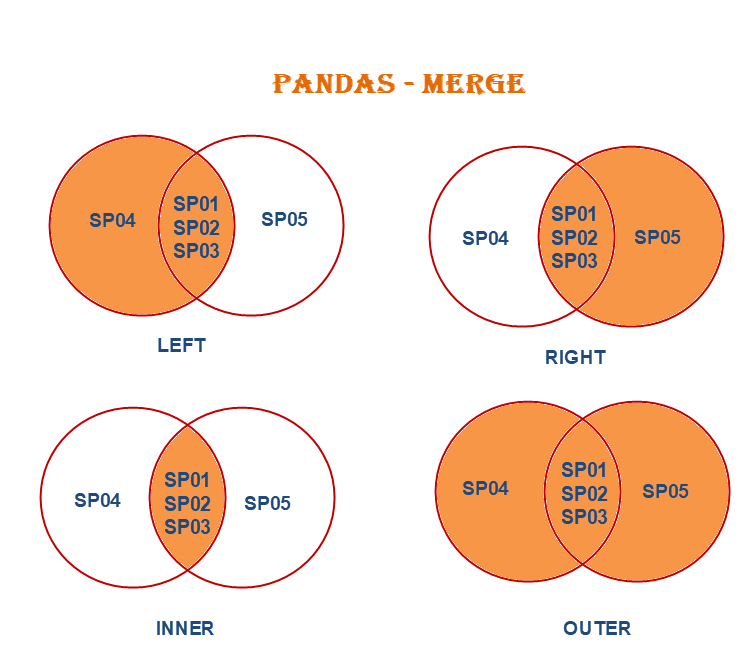
By default, the merge() function in pandas performs an inner join, which combines two DataFrames based on the common keys shared by both. Only the rows with matching keys in both DataFrames are retained in the result.

This behavior can be observed in the following code:

df_enriched_merge = pd.merge(df_existing, df_external, how='inner')
print(df_enriched_merge.shape)
df_enriched_merge.head()

(2, 4)

	FellowshipID	FirstName	Skills	Age
0	1001	Frodo	Hiding	50
1	1002	Samwise	Gardening	39

When you may use inner join? You should use inner join when you cannot carry out the analysis unless the observation corresponding to the key column(s) is present in both the tables.

Example: Suppose you wish to analyze the association between vaccinations and covid infection rate based on country-level data. In one of the datasets, you have the infection rate for each country, while in the other one you have the number of vaccinations in each country. The countries which have either the vaccination or the infection rate missing, cannot help analyze the association. In such as case you may be interested only in countries that have values for both the variables. Thus, you will use inner join to discard the countries with either value missing.

In merge(), the how parameter specifies the type of merge to be performed, the default option is inner, it could also be left, right, and outer.

Description

These join types give you flexibility in how you want to merge and combine data from different sources.

Let’s see how each of these works using our dataframes defined above

Left Join

Returns all rows from the left DataFrame and the matching rows from the right DataFrame.
Missing values (NaN) are introduced for non-matching keys from the right DataFrame.

df_merge_lft = pd.merge(df_existing, df_external, how='left')
print(df_merge_lft.shape)
df_merge_lft.head()

(4, 4)

	FellowshipID	FirstName	Skills	Age
0	1001	Frodo	Hiding	50.0
1	1002	Samwise	Gardening	39.0
2	1003	Gandalf	Spells	NaN
3	1004	Pippin	Fireworks	NaN

When you may use left join? You should use left join when the primary variable(s) of interest are present in the one of the datasets, and whose missing values cannot be imputed. The variable(s) in the other dataset may not be as important or it may be possible to reasonably impute their values, if missing corresponding to the observation in the primary dataset.

Examples:

Suppose you wish to analyze the association between the covid infection rate and the government effectiveness score (a metric used to determine the effectiveness of the government in implementing policies, upholding law and order etc.) based on the data of all countries. Let us say that one of the datasets contains the covid infection rate, while the other one contains the government effectiveness score for each country. If the infection rate for a country is missing, it might be hard to impute. However, the government effectiveness score may be easier to impute based on GDP per capita, crime rate etc. - information that is easily available online. In such a case, you may wish to use a left join where you keep all the countries for which the infection rate is known.
Suppose you wish to analyze the association between demographics such as age, income etc. and the amount of credit card spend. Let us say one of the datasets contains the demographic information of each customer, while the other one contains the credit card spend for the customers who made at least one purchase. In such as case, you may want to do a left join as customers not making any purchase might be absent in the card spend data. Their spend can be imputed as zero after merging the datasets.

Right join

Returns all rows from the right DataFrame and the matching rows from the left DataFrame.
Missing values (NaN) are introduced for non-matching keys from the left DataFrame.

df_merge_right = pd.merge(df_existing, df_external, how='right')
print(df_merge_right.shape)
df_merge_right.head()

(5, 4)

	FellowshipID	FirstName	Skills	Age
0	1001	Frodo	Hiding	50
1	1002	Samwise	Gardening	39
2	1006	Legolas	NaN	2931
3	1007	Elrond	NaN	6520
4	1008	Barromir	NaN	51

When you may use right join? You can always use a left join instead of a right join. Their purpose is the same.

13.2.1.1 outer join

Returns all rows from both DataFrames, with NaN values where no match is found.

df_merge_outer = pd.merge(df_existing, df_external, how='outer')
print(df_merge_outer.shape)
df_merge_outer

(7, 4)

	FellowshipID	FirstName	Skills	Age
0	1001	Frodo	Hiding	50.0
1	1002	Samwise	Gardening	39.0
2	1003	Gandalf	Spells	NaN
3	1004	Pippin	Fireworks	NaN
4	1006	Legolas	NaN	2931.0
5	1007	Elrond	NaN	6520.0
6	1008	Barromir	NaN	51.0

When you may use outer join? You should use an outer join when you cannot afford to lose data present in either of the tables. All the other joins may result in loss of data.

Example: Suppose I took two course surveys for this course. If I need to analyze student sentiment during the course, I will take an outer join of both the surveys. Assume that each survey is a dataset, where each row corresponds to a unique student. Even if a student has answered one of the two surverys, it will be indicative of the sentiment, and will be useful to keep in the merged dataset.

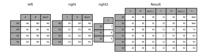
13.2.2 Combining based on Indices: `join()`

Unlike merge(), join() in pandas combines data based on the index. When using join(), you must specify the suffixes parameter if there are overlapping column names, as it does not have default values. You can refer to the official function definition here: pandas.DataFrame.join.

df_enriched_join = df_existing.join(df_external)
print(df_enriched_join.shape)
df_enriched_join.head()

ValueError: columns overlap but no suffix specified: Index(['FellowshipID', 'FirstName'], dtype='object')

Let’s set the suffix to fix this issue

df_enriched_join = df_existing.join(df_external, lsuffix = '_existing',rsuffix = '_external')
print(df_enriched_join.shape)
df_enriched_join.head()

(4, 6)

	FellowshipID_existing	FirstName_existing	Skills	FellowshipID_external	FirstName_external	Age
0	1001	Frodo	Hiding	1001	Frodo	50
1	1002	Samwise	Gardening	1002	Samwise	39
2	1003	Gandalf	Spells	1006	Legolas	2931
3	1004	Pippin	Fireworks	1007	Elrond	6520

As can be observed, join() merges DataFrames using their index and performs a left join.

Now, let’s set the “FellowshipID” column as the index in both DataFrames and see what happens.

# set the index of the dataframes as the "FellowshipID" column
df_existing.set_index('FellowshipID', inplace=True)
df_external.set_index('FellowshipID', inplace=True)

# join the two dataframes
df_enriched_join = df_existing.join(df_external, lsuffix = '_existing',rsuffix = '_external')
print(df_enriched_join.shape)
df_enriched_join

(4, 4)

	FirstName_existing	Skills	FirstName_external	Age
FellowshipID
1001	Frodo	Hiding	Frodo	50.0
1002	Samwise	Gardening	Samwise	39.0
1003	Gandalf	Spells	NaN	NaN
1004	Pippin	Fireworks	NaN	NaN

In this case, df_enriched_join will contain all rows from df_existing and the corresponding matching rows from df_external, with NaN values for non-matching entries.

Similar to merge(), you can change the type of join in join() by explicitly specifying the how parameter. However, this explanation will be skipped here, as the different join types have already been covered in the merge() section above.

13.2.3 Stacking vertically or horizontally: `concat()`

concat() is used in pandas to concatenate DataFrames along a specified axis, either rows or columns. Similar to concat() in NumPy, it defaults to concatenating along the rows.

# let's concatenate the two dataframes using default setting
df_concat = pd.concat([df_existing, df_external])
print(df_concat.shape)
df_concat

(9, 3)

	FirstName	Skills	Age
FellowshipID
1001	Frodo	Hiding	NaN
1002	Samwise	Gardening	NaN
1003	Gandalf	Spells	NaN
1004	Pippin	Fireworks	NaN
1001	Frodo	NaN	50.0
1002	Samwise	NaN	39.0
1006	Legolas	NaN	2931.0
1007	Elrond	NaN	6520.0
1008	Barromir	NaN	51.0

# Concatenating along columns (horizontal)
df_concat_columns = pd.concat([df_existing, df_external], axis=1)
print(df_concat_columns.shape)
df_concat_columns

(7, 4)

	FirstName	Skills	FirstName	Age
FellowshipID
1001	Frodo	Hiding	Frodo	50.0
1002	Samwise	Gardening	Samwise	39.0
1003	Gandalf	Spells	NaN	NaN
1004	Pippin	Fireworks	NaN	NaN
1006	NaN	NaN	Legolas	2931.0
1007	NaN	NaN	Elrond	6520.0
1008	NaN	NaN	Barromir	51.0

13.2.4 Missing values after data enriching

Using either of the approaches mentioned above may introduce missing values for unmatched entries. Handling these missing values is crucial for maintaining the quality and integrity of your dataset after merging or joining DataFrames. It is important to choose a method that best fits your data and analysis goals, and to document your decisions regarding missing value handling for transparency in your analysis.

Question: Read the documentations of the Pandas DataFrame methods merge() and concat(), and identify the differences. Mention examples when you can use (i) either, (ii) only concat(), (iii) only merge()

Solution:

If we need to merge datasets using row indices, we can use either function.
If we need to stack datasets one on top of the other, we can only use concat()
If we need to merge datasets using overlapping columns we can only use merge()

For a comprehensive user guide, please refer to the official documentation.

13.3 Independent Study

13.3.1 Practice exercise 1

You are given the life expectancy data of each continent as a separate *.csv file.

13.3.1.1

Visualize the change of life expectancy over time for different continents.

13.3.1.2

Appending all the data files, i.e., stacking them on top of each other to form a combined datasets called “data_all_continents”

13.3.2 Practice exercise 2

13.3.2.1 Preparing GDP per capita data

Read the GDP per capita data from https://en.wikipedia.org/wiki/List_of_countries_by_GDP_(nominal)_per_capita

Drop all the Year columns. Use the drop() method with the columns, level and inplace arguments. Print the first 2 rows of the updated DataFrame. If the first row of the DataFrame has missing values for all columns, drop that row as well.

13.3.2.2

Drop the inner level of column labels. Use the droplevel() method. Print the first 2 rows of the updated DataFrame.

13.3.2.3

Convert the columns consisting of GDP per capita by IMF, World Bank, and the United Nations to numeric. Apply a lambda function on these columns to convert them to numeric. Print the number of missing values in each column of the updated DataFrame.

Note: Do not apply the function 3 times. Apply it once on a DataFrame consisting of these 3 columns.

13.3.2.4

Apply the lambda function below on all the column names of the dataset obtained in the previous question to clean the column names.

import re

column_name_cleaner = lambda x:re.split(r'\[|/', x)[0]

Note: You will need to edit the parameter of the function, i.e., x in the above function to make sure it is applied on column names and not columns.

Print the first 2 rows of the updated DataFrame.

13.3.2.5

Create a new column GDP_per_capita that copies the GDP per capita values of the United Nations. If the GDP per capita is missing in the United Nations column, then copy it from the World Bank column. If the GDP per capita is missing both in the United Nations and the World Bank columns, then copy it from the IMF column.

Print the number of missing values in the GDP_per_capita column.

13.3.2.6

Drop all the columns except Country and GDP_per_capita. Print the first 2 rows of the updated DataFrame.

13.3.2.7

The country names contain some special characters (characters other than letters) and need to be cleaned. The following function can help clean country names:

import re

country_names_clean_gdp_data = lambda x: re.sub(r'[^\w\s]', '', x).strip()

Apply the above lambda function on the country column to clean country names. Save the cleaned dataset as gdp_per_capita_data. Print the first 2 rows of the updated DataFrame.

13.3.2.8 Preparing population data

Read the population data from https://en.wikipedia.org/wiki/List_of_countries_by_population_(United_Nations).

Drop all columns except Country, UN Continental Region[1], and Population (1 July 2023).
Drop the first row since it is the total population in the world

13.3.2.9

Apply the lambda function below on all the column names of the dataset obtained in the previous question to clean the column names.

import re

column_name_cleaner = lambda x:re.split(r'\[|/|\(| ', x.name)[0]

Note: You will need to edit the parameter of the function, i.e., x in the above function to make sure it is applied on column names and not columns.

Print the first 2 rows of the updated DataFrame.

13.3.2.10

The country names contain some special characters (characters other than letters) and need to be cleaned. The following function can help clean country names:

import re

country_names_clean_population_data = lambda x: re.sub("[\(\[].*?[\)\]]", "", x).strip()

Apply the above lambda function on the country column to clean country names. Save the cleaned dataset as population_data.

13.3.2.11 Merging GDP per capita and population datasets

Merge gdp_per_capita_data with population_data to get the population and GDP per capita of countries in a single dataset. Print the first two rows of the merged DataFrame.

Assume that:

We want to keep the GDP per capita of all countries in the merged dataset, even if their population in unavailable in the population dataset. For countries whose population in unavailable, their Population column will show NA.
We want to discard an observation of a country if its GDP per capita is unavailable.

13.3.2.12

For how many countries in gdp_per_capita_data does the population seem to be unavailable in population_data? Note that you don’t need to clean country names any further than cleaned by the functions provided.

Print the observations of gdp_per_capita_data with missing Population.

13.3.3 Merging datasets with similar values in the key column

We suspect that population of more countries may be available in population_data. However, due to unclean country names, the observations could not merge. For example, the country Guinea Bissau is mentioned as GuineaBissau in gdp_per_capita_data and Guinea-Bissau in population_data. To resolve this issue, we’ll use a different approach to merge datasts. We’ll merge the population of a country to an observation in the GDP per capita dataset, whose name in population_data is the most ‘similar’ to the name of the country in gdp_per_capita_data.

13.3.3.1

Proceed as follows:

For each country in gdp_per_capita_data, find the country with the most ‘similar’ name in population_data, based on the similarity score. Use the lambda function provided below to compute the similarity score between two strings (The higher the score, the more similar are the strings. The similarity score is \(1.0\) if two strings are exactly the same).
Merge the population of the most ‘similar’ country to the country in gdp_per_capita_data. The merged dataset must include 5 columns - the country name as it appears in gdp_per_capita_data, the GDP per capita, the country name of the most ‘similar’ country as it appears in population_data, the population of that country, and the similarity score between the country names.
After creating the merged dataset, print the rows of the dataset that have similarity scores less than 1.

Use the function below to compute the similarity score between the Country names of the two datasets:

from difflib import SequenceMatcher

similar = lambda a,b: SequenceMatcher(None, a, b).ratio()

Note: You may use one for loop only for this particular question. However, it would be perfect if don’t use a for loop

Hint:

Define a function that computes the index of the observation having the most ‘similar’ country name in population_data for an observation in gdp_per_capita_data. The function returns a Series consisting of the most ‘similar’ country name, its population, and its similarity score (This function can be written with only one line in its body, excluding the return statement and the definition statement. However, you may use as many lines as you wish).
Apply the function on the Country column of gdp_per_capita_data. A DataFrame will be obtained.
Concatenate the DataFrame obtained in (2) with gdp_per_capita_data with the pandas concat() function.

13.3.3.2

In the dataset obtained in the previous question, for all observations where similarity score is less than 0.8, replace the population with Nan.

Print the observations of the dataset having missing values of population.

13.1 Data Reshaping

13.1.1 Why Data Reshaping is Important:

13.1.2 Wide vs. Long Data Format in Data Reshaping

13.1.3 Pivoting “long” to “wide” using pivot_table()

13.1.3.1 Pivoting a single column

13.1.4 Melting “wide” to “long” using melt()

13.1.5 Stacking and Unstacking using stack() and unstack()

13.1.5.1 Understanding the level in multi-level index and columns

13.1.5.2 Stacking (Columns to Rows ): stack()

13.1.5.3 Unstacking (Rows to Columns) : unstack()

13.1.6 Transposing using .T attribute

13.1.7 Summary of Common Reshaping Functions

13.1.8 Converting from Multi-Level Index to Single-Level Index DataFrame

13.2 Data Enriching

13.2.1 Combining based on common keys: merge()

13.2.1.1 outer join

13.2.2 Combining based on Indices: join()

13.2.3 Stacking vertically or horizontally: concat()

13.2.4 Missing values after data enriching

13.3 Independent Study

13.3.1 Practice exercise 1

13.3.1.1

13.3.1.2

13.3.2 Practice exercise 2

13.3.2.1 Preparing GDP per capita data

13.3.2.2

13.3.2.3

13.3.2.4

13.3.2.5

13.3.2.6

13.3.2.7

13.3.2.8 Preparing population data

13.3.2.9

13.3.2.10

13.3.2.11 Merging GDP per capita and population datasets

13.3.2.12

13.3.3 Merging datasets with similar values in the key column

13.3.3.1

13.3.3.2

13.1.3 Pivoting “long” to “wide” using `pivot_table()`

13.1.4 Melting “wide” to “long” using `melt()`

13.1.5 Stacking and Unstacking using `stack()` and `unstack()`

13.1.5.1 Understanding the `level` in multi-level index and columns

13.1.5.2 Stacking (Columns to Rows ): `stack()`

13.1.5.3 Unstacking (Rows to Columns) : `unstack()`

13.1.6 Transposing using `.T` attribute

13.2.1 Combining based on common keys: `merge()`

13.2.2 Combining based on Indices: `join()`

13.2.3 Stacking vertically or horizontally: `concat()`