7  Pandas Fundamentals

7.1 Introduction to Pandas Fundamentals

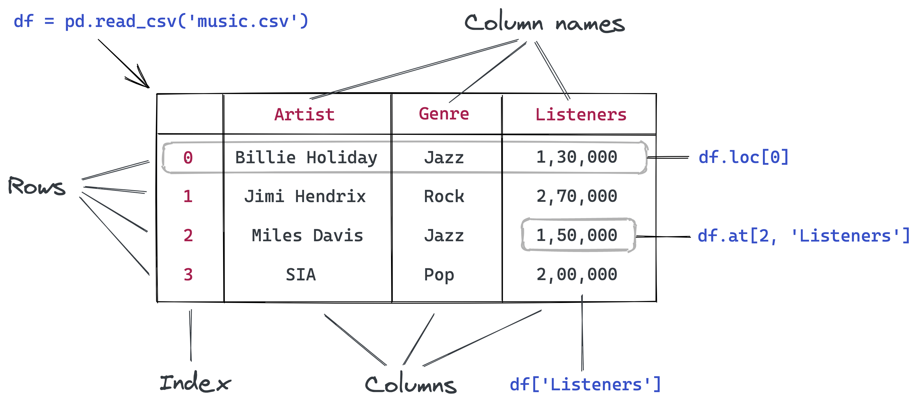
In the Reading Data chapter, we learned how to load data files into pandas DataFrames. Now we’ll dive deeper into pandas’ powerful capabilities for data manipulation and analysis.

Pandas is an essential tool in the data scientist or data analyst’s toolkit due to its ability to handle and transform data with ease and efficiency.

7.1.1 Pandas in the Data Science Ecosystem

Pandas doesn’t work in isolation - it’s designed to integrate seamlessly with other Python libraries:

Library	Integration with Pandas	Purpose
NumPy	Built on NumPy arrays	Mathematical operations and array processing
Matplotlib	Direct plotting from DataFrames	Data visualization and charts
Seaborn	Native DataFrame support	Statistical visualizations
Scikit-learn	Seamless data flow	Machine learning algorithms
SciPy	Statistical analysis	Advanced statistical functions

7.1.2 Core Pandas Capabilities

Throughout this chapter, you’ll master these essential pandas operations:

• Creating Series & DataFrames: From Python data structures
  
• Filtering & Subsetting: Extract exactly the data you need
  
• Sorting & Ranking: Organize data for analysis
  
• Adding & Removing: Modify DataFrame structure
  
• Data Types: Work with different types of data

💡 Learning Path: We’ll start with fundamental concepts and progressively build toward advanced data manipulation techniques, giving you a complete toolkit for real-world data analysis.

Now let’s start by importing the essential Pandas library:

import pandas as pd

7.2 Creating Pandas Series & DataFrames

There are two primary approaches for creating pandas data structures, each serving different purposes in your data analysis workflow:

7.2.1 Method 1: Reading from External Data Sources

In real-world data science, you’ll typically work with data stored in external files or databases. This is the most common approach for production analysis.

Popular Data Sources:

Source Type	Pandas Function	Use Case
CSV Files	pd.read_csv()	Most common - structured tabular data
Excel Files	pd.read_excel()	Business data, reports with multiple sheets
JSON Files	pd.read_json()	API data, web services, nested data
SQL Databases	pd.read_sql()	Enterprise databases, large datasets
HTML Tables	pd.read_html()	Web scraping, online data tables

💡 Pro Tip: We covered these methods extensively in the Reading Data chapter. If you need a refresher on loading external data, refer back to that section!

7.2.2 Method 2: Creating from Python Data Structures

When you need to create data programmatically or work with small datasets for testing and learning, you can build DataFrames and Series directly from Python objects.

Benefits of this approach:

• Testing & Learning: Perfect for experimenting with pandas features
• Data Generation: Create synthetic data for analysis
• Small Datasets: Handle simple, manual data entry
• Prototyping: Quick data structure creation for proof-of-concepts

Let’s explore how to create pandas data structures from scratch!

7.2.2.1 Creating Series from Python Data Structures

A Series is pandas’ 1D data structure - think of it as a smart, labeled list or array.

7.2.2.1.1 Method A: From a Python List

The simplest way to create a Series is from a Python list. Pandas automatically assigns integer indices starting from 0.

#Defining a Pandas Series
series_example = pd.Series(['these','are','english','words'])
series_example

0      these
1        are
2    english
3      words
dtype: object

🔍 Key Observation: Notice the automatic integer indices (0, 1, 2, 3) on the left!

Custom Indexing: You can provide meaningful labels instead of default numbers using the index parameter:

#Defining a Pandas Series with custom row labels
series_example = pd.Series(['these','are','english','words'], index = range(101,105))
series_example

101      these
102        are
103    english
104      words
dtype: object

7.2.2.1.2 Method B: From a Python Dictionary

Dictionaries are perfect for creating Series with meaningful labels. The dictionary keys automatically become the Series index, and values become the data points.

Perfect for: Time series data, named categories, any key-value relationships

# 📊 Real-world example: US GDP per capita by year (1960-2021)
# Notice some years are missing - pandas handles this gracefully!
GDP_per_capita_dict = {'1960':3007,'1961':3067,'1962':3244,'1963':3375,'1964':3574,'1965':3828,'1966':4146,'1967':4336,'1968':4696,'1970':5234,'1971':5609,'1972':6094,'1973':6726,'1974':7226,'1975':7801,'1976':8592,'1978':10565,'1979':11674, '1980':12575,'1981':13976,'1982':14434,'1983':15544,'1984':17121,'1985':18237,  '1986':19071,'1987':20039,'1988':21417,'1989':22857,'1990':23889,'1991':24342,  '1992':25419,'1993':26387,'1994':27695,'1995':28691,'1996':29968,'1997':31459,  '1998':32854,'2000':36330,'2001':37134,'2002':37998,'2003':39490,'2004':41725,  '2005':44123,'2006':46302,'2007':48050,'2008':48570,'2009':47195,'2010':48651,  '2011':50066,'2012':51784,'2013':53291,'2015':56763,'2016':57867,'2017':59915,'2018':62805, '2019':65095,'2020':63028,'2021':69288}

#Example 2: Creating a Pandas Series from a Dictionary
GDP_per_capita_series = pd.Series(GDP_per_capita_dict)
GDP_per_capita_series.head()

1960    3007
1961    3067
1962    3244
1963    3375
1964    3574
dtype: int64

7.2.2.2 Creating a DataFrame from Python Data Structures

7.2.2.2.1 Method A: From a list of Python Dictionary

You can create a DataFrame where keys are column names and values are lists representing column data.

#List of dictionary consisting of 52 playing cards of the deck
deck_list_of_dictionaries = [{'value':i, 'suit':c}
for c in ['spades', 'clubs', 'hearts', 'diamonds']
for i in range(2,15)]

#Example 3: Creating a Pandas DataFrame from a List of dictionaries
deck_df = pd.DataFrame(deck_list_of_dictionaries)
deck_df.head()

	value	suit
0	2	spades
1	3	spades
2	4	spades
3	5	spades
4	6	spades

7.2.2.2.2 Method B: From a Python Dictionary

You can create a DataFrame where keys are column names and values are lists representing column data.

#Example 4: Creating a Pandas DataFrame from a Dictionary
dict_data = {'A': [1, 2, 3, 4, 5],
        'B': [20, 10, 50, 40, 30],
        'C': [100, 200, 300, 400, 500]}

dict_df = pd.DataFrame(dict_data)
dict_df

	A	B	C
0	1	20	100
1	2	10	200
2	3	50	300
3	4	40	400
4	5	30	500

7.3 Data Selection and Filtering

Now that you understand series and dataframe are two foundamental data structures in pandas, let’s master the art of extracting exactly the data you need. Data selection and filtering are fundamental skills that you’ll use in every pandas project.

7.3.1 Basic Selection

7.3.1.1 Extracting Column(s)

The first step when working with a DataFrame is often to extract one or more columns. To do this effectively, it’s helpful to understand the internal structure of a DataFrame. Conceptually, you can think of a DataFrame as a dictionary of lists, where the keys are column names, and the values are lists or arrays containing data for the respective columns.

Loading Our Practice Dataset

Let’s work with a real movie ratings dataset to practice our selection techniques:

import pandas as pd
movie_ratings = pd.read_csv('./datasets/movie_ratings.csv')
movie_ratings.head()

	Title	US Gross	Worldwide Gross	Production Budget	Release Date	MPAA Rating	Source	Major Genre	Creative Type	IMDB Rating	IMDB Votes
0	Opal Dreams	14443	14443	9000000	Nov 22 2006	PG/PG-13	Adapted screenplay	Drama	Fiction	6.5	468
1	Major Dundee	14873	14873	3800000	Apr 07 1965	PG/PG-13	Adapted screenplay	Western/Musical	Fiction	6.7	2588
2	The Informers	315000	315000	18000000	Apr 24 2009	R	Adapted screenplay	Horror/Thriller	Fiction	5.2	7595
3	Buffalo Soldiers	353743	353743	15000000	Jul 25 2003	R	Adapted screenplay	Comedy	Fiction	6.9	13510
4	The Last Sin Eater	388390	388390	2200000	Feb 09 2007	PG/PG-13	Adapted screenplay	Drama	Fiction	5.7	1012

7.3.1.1.1 Method 1: Single Column Extraction

Each column represents a feature of your data. There are two ways to extract a single column:

A) Bracket Notation: df['column_name'] (Recommended)

• ✅ Always works
  
• ✅ Handles column names with spaces
• ✅ Clear and explicit

B) Dot Notation: df.column_name (Limited use)

• ❌ Fails with spaces in column names
• ❌ Conflicts with DataFrame methods
• ✅ Shorter syntax for simple names

movie_ratings.Title

0                         Opal Dreams
1                        Major Dundee
2                       The Informers
3                    Buffalo Soldiers
4                  The Last Sin Eater
                    ...              
2223                      King Arthur
2224                            Mulan
2225                       Robin Hood
2226    Robin Hood: Prince of Thieves
2227                       Spiceworld
Name: Title, Length: 2228, dtype: object

# 🧠 Understanding the DataFrame structure: 
# DataFrames work like dictionaries with enhanced features!
movie_ratings_dict = {
    'Title':  ['Opal Dreams', 'Major Dundee', 'The Informers', 'Buffalo Soldiers', 'The Last Sin Eater'],
    'US Gross':  [14443, 14873, 315000, 353743, 388390],
    'Worldwide Gross': [14443, 14873, 315000, 353743, 388390],
    'Production Budget': [9000000, 3800000, 18000000, 15000000, 2200000]
}

Dictionary Analogy:

Just like accessing dictionary values by key:

movie_ratings_dict['Title']

['Opal Dreams',
 'Major Dundee',
 'The Informers',
 'Buffalo Soldiers',
 'The Last Sin Eater']

DataFrame Column Extraction:

Similarly, we extract DataFrame columns by column name:

movie_ratings['Title']

0                         Opal Dreams
1                        Major Dundee
2                       The Informers
3                    Buffalo Soldiers
4                  The Last Sin Eater
                    ...              
2223                      King Arthur
2224                            Mulan
2225                       Robin Hood
2226    Robin Hood: Prince of Thieves
2227                       Spiceworld
Name: Title, Length: 2228, dtype: object

7.3.1.1.2 Method 2: Multiple Column Selection

Key Rule: Use a list of column names inside the brackets:

# Single column → Series
df['column']        

# Multiple columns → DataFrame  
df[['col1', 'col2']]

🔍 Notice: Double brackets [[]] create a list, which tells pandas you want multiple columns!

movie_ratings[['Title', 'US Gross', 'Worldwide Gross' ]]

	Title	US Gross	Worldwide Gross
0	Opal Dreams	14443	14443
1	Major Dundee	14873	14873
2	The Informers	315000	315000
3	Buffalo Soldiers	353743	353743
4	The Last Sin Eater	388390	388390
...	...	...	...
2223	King Arthur	51877963	203877963
2224	Mulan	120620254	303500000
2225	Robin Hood	105269730	310885538
2226	Robin Hood: Prince of Thieves	165493908	390500000
2227	Spiceworld	29342592	56042592

2228 rows × 3 columns

7.3.1.2 Extracting Row(s)

In many cases, we need to filter rows based on specific conditions or a combination of multiple conditions. Next, let’s explore how to use these conditions effectively to extract rows that meet our criteria, whether it’s a single condition or multiple conditions combined

7.3.1.2.1 Single Condition Filtering

Filter rows in a DataFrame based on one logical condition.
This is the most common way to extract a subset of data, such as selecting all rows where a column’s values meet a specific criterion (e.g., greater than, equal to, not equal).

For Example:

# extracting the rows that have IMDB Rating greater than 8
movie_ratings[movie_ratings['IMDB Rating'] > 8]

	Title	US Gross	Worldwide Gross	Production Budget	Release Date	MPAA Rating	Source	Major Genre	Creative Type	IMDB Rating	IMDB Votes
21	Gandhi, My Father	240425	1375194	5000000	Aug 03 2007	Other	Adapted screenplay	Drama	Non-Fiction	8.1	50881
56	Ed Wood	5828466	5828466	18000000	Sep 30 1994	R	Adapted screenplay	Comedy	Non-Fiction	8.1	74171
67	Requiem for a Dream	3635482	7390108	4500000	Oct 06 2000	Other	Adapted screenplay	Drama	Fiction	8.5	185226
164	Trainspotting	16501785	24000785	3100000	Jul 19 1996	R	Adapted screenplay	Drama	Fiction	8.2	150483
181	The Wizard of Oz	28202232	28202232	2777000	Aug 25 2039	G	Adapted screenplay	Western/Musical	Fiction	8.3	102795
...	...	...	...	...	...	...	...	...	...	...	...
2090	Finding Nemo	339714978	867894287	94000000	May 30 2003	G	Original Screenplay	Action/Adventure	Fiction	8.2	165006
2092	Toy Story 3	410640665	1046340665	200000000	Jun 18 2010	G	Original Screenplay	Action/Adventure	Fiction	8.9	67380
2094	Avatar	760167650	2767891499	237000000	Dec 18 2009	PG/PG-13	Original Screenplay	Action/Adventure	Fiction	8.3	261439
2130	Scarface	44942821	44942821	25000000	Dec 09 1983	Other	Adapted screenplay	Drama	Fiction	8.2	152262
2194	The Departed	133311000	290539042	90000000	Oct 06 2006	R	Adapted screenplay	Drama	Fiction	8.5	264148

97 rows × 11 columns

7.3.1.2.2 Multiple Conditions Filtering

When filtering with more than one condition, use logical operators:

Operator	Purpose	Example
&	AND – both conditions must be True	(df['A'] > 5) & (df['B'] < 10)
\|	OR – at least one condition must be True	(df['A'] > 5) \| (df['B'] < 10)
~	NOT – negates the condition	~(df['A'] > 5)

🚨 Important Rule: Always wrap each condition in parentheses () to avoid operator precedence errors.

# extracting the rows that have IMDB Rating greater than 8 and US Gross less than 1000000
movie_ratings[(movie_ratings['IMDB Rating'] > 8) & (movie_ratings['US Gross'] < 1000000)]

	Title	US Gross	Worldwide Gross	Production Budget	Release Date	MPAA Rating	Source	Major Genre	Creative Type	IMDB Rating	IMDB Votes
21	Gandhi, My Father	240425	1375194	5000000	Aug 03 2007	Other	Adapted screenplay	Drama	Non-Fiction	8.1	50881
636	Lake of Fire	25317	25317	6000000	Oct 03 2007	Other	Adapted screenplay	Documentary	Non-Fiction	8.4	1027

7.3.1.2.3 Negating Conditions with the ~ Operator

The tilde (~) operator in pandas is used to negate boolean conditions, making it especially useful when you want to exclude certain rows.

Instead of selecting rows that satisfy a condition, ~ allows you to filter rows that do not meet that condition. This is helpful for refining queries and focusing on the remaining data.

For example, if you want all rows where IMDB Rating is not equal to 8, you can write:

# Excluding the rows that have IMDB Rating that equals 8 using the tilde ~
movie_ratings[~(movie_ratings['IMDB Rating'] == 8)]

	Title	US Gross	Worldwide Gross	Production Budget	Release Date	MPAA Rating	Source	Major Genre	Creative Type	IMDB Rating	IMDB Votes
0	Opal Dreams	14443	14443	9000000	Nov 22 2006	PG/PG-13	Adapted screenplay	Drama	Fiction	6.5	468
1	Major Dundee	14873	14873	3800000	Apr 07 1965	PG/PG-13	Adapted screenplay	Western/Musical	Fiction	6.7	2588
2	The Informers	315000	315000	18000000	Apr 24 2009	R	Adapted screenplay	Horror/Thriller	Fiction	5.2	7595
3	Buffalo Soldiers	353743	353743	15000000	Jul 25 2003	R	Adapted screenplay	Comedy	Fiction	6.9	13510
4	The Last Sin Eater	388390	388390	2200000	Feb 09 2007	PG/PG-13	Adapted screenplay	Drama	Fiction	5.7	1012
...	...	...	...	...	...	...	...	...	...	...	...
2223	King Arthur	51877963	203877963	90000000	Jul 07 2004	PG/PG-13	Adapted screenplay	Action/Adventure	Fiction	6.2	53106
2224	Mulan	120620254	303500000	90000000	Jun 19 1998	G	Adapted screenplay	Action/Adventure	Non-Fiction	7.2	34256
2225	Robin Hood	105269730	310885538	210000000	May 14 2010	PG/PG-13	Adapted screenplay	Action/Adventure	Fiction	6.9	34501
2226	Robin Hood: Prince of Thieves	165493908	390500000	50000000	Jun 14 1991	PG/PG-13	Adapted screenplay	Action/Adventure	Fiction	6.7	54480
2227	Spiceworld	29342592	56042592	25000000	Jan 23 1998	PG/PG-13	Adapted screenplay	Comedy	Fiction	2.9	18010

2191 rows × 11 columns

Alternative: Using !=

Another way to exclude rows where a column equals a certain value is to use the not-equal operator !=:

# using the != operator
movie_ratings[movie_ratings['IMDB Rating'] != 8]

	Title	US Gross	Worldwide Gross	Production Budget	Release Date	MPAA Rating	Source	Major Genre	Creative Type	IMDB Rating	IMDB Votes
0	Opal Dreams	14443	14443	9000000	Nov 22 2006	PG/PG-13	Adapted screenplay	Drama	Fiction	6.5	468
1	Major Dundee	14873	14873	3800000	Apr 07 1965	PG/PG-13	Adapted screenplay	Western/Musical	Fiction	6.7	2588
2	The Informers	315000	315000	18000000	Apr 24 2009	R	Adapted screenplay	Horror/Thriller	Fiction	5.2	7595
3	Buffalo Soldiers	353743	353743	15000000	Jul 25 2003	R	Adapted screenplay	Comedy	Fiction	6.9	13510
4	The Last Sin Eater	388390	388390	2200000	Feb 09 2007	PG/PG-13	Adapted screenplay	Drama	Fiction	5.7	1012
...	...	...	...	...	...	...	...	...	...	...	...
2223	King Arthur	51877963	203877963	90000000	Jul 07 2004	PG/PG-13	Adapted screenplay	Action/Adventure	Fiction	6.2	53106
2224	Mulan	120620254	303500000	90000000	Jun 19 1998	G	Adapted screenplay	Action/Adventure	Non-Fiction	7.2	34256
2225	Robin Hood	105269730	310885538	210000000	May 14 2010	PG/PG-13	Adapted screenplay	Action/Adventure	Fiction	6.9	34501
2226	Robin Hood: Prince of Thieves	165493908	390500000	50000000	Jun 14 1991	PG/PG-13	Adapted screenplay	Action/Adventure	Fiction	6.7	54480
2227	Spiceworld	29342592	56042592	25000000	Jan 23 1998	PG/PG-13	Adapted screenplay	Comedy	Fiction	2.9	18010

2191 rows × 11 columns

7.3.2 Advanced Selection: .loc[] and .iloc[]

When you need precise control over both rows and columns, pandas provides two powerful indexers that let you select exactly what you need.

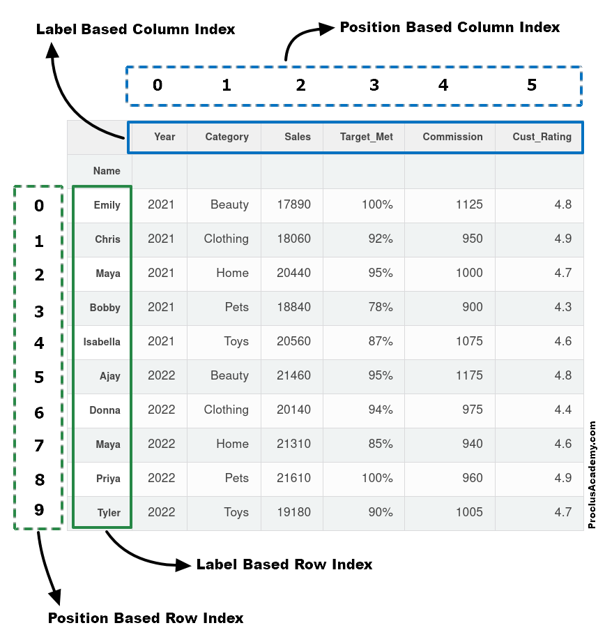
7.3.2.1 .loc[] vs .iloc[]: The Key Difference

Indexer	Uses	Best For	Example
.loc[]	Labels (names)	Human-readable selection	df.loc['row_name', 'column_name']
.iloc[]	Positions (numbers)	Programmatic selection	df.iloc[0, 1]

Mental Model

Think of your DataFrame like a spreadsheet:

• .loc[] works like clicking on named rows/columns (A1, B2, etc.)
• .iloc[] works like clicking on position numbers (row 0, column 1, etc.)

💡 Memory Tip:

• loc = Labels/Location names
• iloc = integer locations

Preparing Our Data: Sorting by IMDB Rating

To demonstrate .loc[] and .iloc[] effectively, let’s first sort our movies by rating so we can easily select the best ones:

movie_ratings_sorted = movie_ratings.sort_values(by = 'IMDB Rating', ascending = False)
movie_ratings_sorted.head()

	Title	US Gross	Worldwide Gross	Production Budget	Release Date	MPAA Rating	Source	Major Genre	Creative Type	IMDB Rating	IMDB Votes
182	The Shawshank Redemption	28241469	28241469	25000000	Sep 23 1994	R	Adapted screenplay	Drama	Fiction	9.2	519541
2084	Inception	285630280	753830280	160000000	Jul 16 2010	PG/PG-13	Original Screenplay	Horror/Thriller	Fiction	9.1	188247
790	Schindler's List	96067179	321200000	25000000	Dec 15 1993	R	Adapted screenplay	Drama	Non-Fiction	8.9	276283
1962	Pulp Fiction	107928762	212928762	8000000	Oct 14 1994	R	Original Screenplay	Drama	Fiction	8.9	417703
561	The Dark Knight	533345358	1022345358	185000000	Jul 18 2008	PG/PG-13	Adapted screenplay	Action/Adventure	Fiction	8.9	465000

7.3.2.2 Using .loc[] - Label-Based Selection

Syntax: df.loc[row_indexer, column_indexer]

Key Features:

• Uses actual labels (index names, column names)
• Inclusive of both endpoints in slicing
• Can combine with boolean conditions
• Most intuitive for data analysis

Example: Let’s subset the Title, Worldwide Gross, Production Budget, and IMDB Rating of the top 3 movies using specific row indices that obtained from the above sorting table.

# 📍 Select specific rows by index and specific columns by name
movies_subset = movie_ratings_sorted.loc[[182, 2084, 790], ['Title', 'IMDB Rating', 'US Gross', 'Worldwide Gross', 'Production Budget']]
print("🎬 Selected movies with key financial and rating data:")
movies_subset

🎬 Selected movies with key financial and rating data:

	Title	IMDB Rating	US Gross	Worldwide Gross	Production Budget
182	The Shawshank Redemption	9.2	28241469	28241469	25000000
2084	Inception	9.1	285630280	753830280	160000000
790	Schindler's List	8.9	96067179	321200000	25000000

The : symbol in .loc is a slicing operator that represents a range or all elements in the specified dimension (rows or columns). Use : alone to select all rows/columns, or with start/end points to slice specific parts of the DataFrame.

# 📊 Select ALL rows (:) but only specific columns
movies_subset = movie_ratings_sorted.loc[:, ['Title', 'Worldwide Gross', 'Production Budget', 'IMDB Rating']]
print(" All movies with financial and rating columns only:")
movies_subset

 All movies with financial and rating columns only:

	Title	Worldwide Gross	Production Budget	IMDB Rating
182	The Shawshank Redemption	28241469	25000000	9.2
2084	Inception	753830280	160000000	9.1
790	Schindler's List	321200000	25000000	8.9
1962	Pulp Fiction	212928762	8000000	8.9
561	The Dark Knight	1022345358	185000000	8.9
...	...	...	...	...
1051	Glitter	4273372	8500000	2.0
1495	Disaster Movie	34690901	20000000	1.7
1116	Crossover	7009668	5600000	1.7
805	From Justin to Kelly	4922166	12000000	1.6
1147	Super Babies: Baby Geniuses 2	9109322	20000000	1.4

2228 rows × 4 columns

# 📏 Select a RANGE of rows (182 to 561) and specific columns
movies_subset = movie_ratings_sorted.loc[182:561, ['Title', 'Worldwide Gross', 'Production Budget', 'IMDB Rating']]
print("Movies from index 182 to 561 (inclusive):")
movies_subset

Movies from index 182 to 561 (inclusive):

	Title	Worldwide Gross	Production Budget	IMDB Rating
182	The Shawshank Redemption	28241469	25000000	9.2
2084	Inception	753830280	160000000	9.1
790	Schindler's List	321200000	25000000	8.9
1962	Pulp Fiction	212928762	8000000	8.9
561	The Dark Knight	1022345358	185000000	8.9

7.3.2.3 Combining .loc with Boolean Conditions

Power Move: Filter rows AND select columns simultaneously using boolean logic!

# extracting the rows that have IMDB Rating greater than 8 or US Gross less than 1000000, only extract the Title and IMDB Rating columns
movie_ratings[(movie_ratings['IMDB Rating'] > 8) & (movie_ratings['US Gross'] < 1000000)][['Title','IMDB Rating']]

#using loc to extract the rows that have IMDB Rating greater than 8 or US Gross less than 1000000, only extract the Title and IMDB Rating columns
movie_ratings.loc[(movie_ratings['IMDB Rating'] > 8) & (movie_ratings['US Gross'] < 1000000),['Title','IMDB Rating']]

	Title	IMDB Rating
21	Gandhi, My Father	8.1
636	Lake of Fire	8.4

7.3.2.4 Using .iloc[] - Position-Based Selection

Syntax: df.iloc[row_positions, column_positions]

Key Features:

• Uses integer positions (0-based indexing like Python lists)
• Exclusive of end point in slicing (like Python slicing)
• Great for systematic sampling or first/last N records
• Think: integer location

Position Type	Example	Description
Single	df.iloc[0, 1]	First row, second column
List	df.iloc[[0, 2], [1, 3]]	Specific positions
Slice	df.iloc[0:3, 1:4]	Range (exclusive end)
All	df.iloc[:, :]	All rows and columns

💡 Memory Tip:

• iloc = integer positions,
• loc = label names

# let's check  the movie_ratings_sorted DataFrame
movie_ratings_sorted.head()

	Title	US Gross	Worldwide Gross	Production Budget	Release Date	MPAA Rating	Source	Major Genre	Creative Type	IMDB Rating	IMDB Votes
182	The Shawshank Redemption	28241469	28241469	25000000	Sep 23 1994	R	Adapted screenplay	Drama	Fiction	9.2	519541
2084	Inception	285630280	753830280	160000000	Jul 16 2010	PG/PG-13	Original Screenplay	Horror/Thriller	Fiction	9.1	188247
790	Schindler's List	96067179	321200000	25000000	Dec 15 1993	R	Adapted screenplay	Drama	Non-Fiction	8.9	276283
1962	Pulp Fiction	107928762	212928762	8000000	Oct 14 1994	R	Original Screenplay	Drama	Fiction	8.9	417703
561	The Dark Knight	533345358	1022345358	185000000	Jul 18 2008	PG/PG-13	Adapted screenplay	Action/Adventure	Fiction	8.9	465000

After sorting, the position-based index changes, while the label-based index remains unchanged. Let’s pass the position-based index to iloc to retrieve the top 2 rows from the movie_ratings_sorted DataFrame.

# 🏆 Get first 2 rows by POSITION (0 and 1), all columns
top_2_movies = movie_ratings_sorted.iloc[0:2, :]
print(" Top 2 movies by position:")
top_2_movies

 Top 2 movies by position:

	Title	US Gross	Worldwide Gross	Production Budget	Release Date	MPAA Rating	Source	Major Genre	Creative Type	IMDB Rating	IMDB Votes
182	The Shawshank Redemption	28241469	28241469	25000000	Sep 23 1994	R	Adapted screenplay	Drama	Fiction	9.2	519541
2084	Inception	285630280	753830280	160000000	Jul 16 2010	PG/PG-13	Original Screenplay	Horror/Thriller	Fiction	9.1	188247

It is important to note that the endpoint is excluded in an iloc slice.

For comparison, let’s pass the same argument to loc and see what it returns.

# 🔍 Same range [0:2] with loc - uses LABELS, includes endpoint
loc_result = movie_ratings_sorted.loc[0:2, :]
print(" Using .loc[0:2,:] - includes rows with labels 0, 1, AND 2:")
loc_result

 Using .loc[0:2,:] - includes rows with labels 0, 1, AND 2:

	Title	US Gross	Worldwide Gross	Production Budget	Release Date	MPAA Rating	Source	Major Genre	Creative Type	IMDB Rating	IMDB Votes
0	Opal Dreams	14443	14443	9000000	Nov 22 2006	PG/PG-13	Adapted screenplay	Drama	Fiction	6.5	468
851	Star Trek: Generations	75671262	120000000	38000000	Nov 18 1994	PG/PG-13	Adapted screenplay	Action/Adventure	Fiction	6.5	26465
140	Tuck Everlasting	19161999	19344615	15000000	Oct 11 2002	PG/PG-13	Adapted screenplay	Drama	Fiction	6.5	6639
708	De-Lovely	13337299	18396382	4000000	Jun 25 2004	PG/PG-13	Adapted screenplay	Drama	Fiction	6.5	6086
705	Flyboys	13090630	14816379	60000000	Sep 22 2006	PG/PG-13	Adapted screenplay	Drama	Non-Fiction	6.5	13934
...	...	...	...	...	...	...	...	...	...	...	...
955	The Brothers Solomon	900926	900926	10000000	Sep 07 2007	R	Original Screenplay	Comedy	Fiction	5.2	6044
1637	Drumline	56398162	56398162	20000000	Dec 13 2002	PG/PG-13	Original Screenplay	Comedy	Fiction	5.2	18165
1610	Hollywood Homicide	30207785	51107785	75000000	Jun 13 2003	PG/PG-13	Original Screenplay	Action/Adventure	Fiction	5.2	16452
569	Doom	28212337	54612337	70000000	Oct 21 2005	R	Adapted screenplay	Horror/Thriller	Fiction	5.2	39473
2	The Informers	315000	315000	18000000	Apr 24 2009	R	Adapted screenplay	Horror/Thriller	Fiction	5.2	7595

812 rows × 11 columns

As you can see, : is used in the same way as in loc to denote a range of the index. All rows between label indices 0 and 2, inclusive of both ends, are returned.

# 🎯 Select first 10 rows and specific column positions [0, 2, 3, 9]
movies_iloc_subset = movie_ratings_sorted.iloc[0:10, [0, 2, 3, 9]]
print("📋 First 10 movies with columns at positions 0, 2, 3, 9:")
movies_iloc_subset

📋 First 10 movies with columns at positions 0, 2, 3, 9:

	Title	Worldwide Gross	Production Budget	IMDB Rating
182	The Shawshank Redemption	28241469	25000000	9.2
2084	Inception	753830280	160000000	9.1
790	Schindler's List	321200000	25000000	8.9
1962	Pulp Fiction	212928762	8000000	8.9
561	The Dark Knight	1022345358	185000000	8.9
2092	Toy Story 3	1046340665	200000000	8.9
487	The Lord of the Rings: The Fellowship of the Ring	868621686	109000000	8.8
335	Fight Club	100853753	65000000	8.8
497	The Lord of the Rings: The Return of the King	1133027325	94000000	8.8
1081	C'era una volta il West	5321508	5000000	8.8

🤔 Critical Thinking Question: Can you use .iloc for conditional filtering (like df.iloc[df['column'] > 5])?

Answer: ❌ No! .iloc only accepts integer positions, not boolean conditions. For conditional filtering, you must use .loc or boolean indexing directly.

7.3.2.5 Summary: .loc vs .iloc - Choose Your Weapon!

Feature	.loc (Label-Based)	.iloc (Position-Based)
Uses	🏷️ Labels/Names	🔢 Integer Positions
Slicing	[start:end] includes end	[start:end] excludes end
Examples	df.loc['row_name', 'col_name']	df.iloc[0, 1]
Conditions	✅ df.loc[df['col'] > 5]	❌ No boolean conditions
Best For	Business logic filtering	Systematic sampling

Mental Model:

• .loc = Give me the data by name/label
• .iloc = Give me the data by position number

7.3.3 Finding Extremes in pandas: Values, Labels, and Positions

7.3.3.1 Finding extreme values

When you need to find extreme values, pandas offers powerful methods:

Method	Purpose	Returns
min()	📉 Actual minimum value	The minimum value itself
max()	📈 Actual maximum value	The maximum value itself

# find the max/min worldwide gross
max_gross = max(movie_ratings["Worldwide Gross"])
min_gross = min(movie_ratings["Worldwide Gross"])

print("Hignest gross:", max_gross)
print("Minimum gross:", min_gross)

Hignest gross: 2767891499
Minimum gross: 884

7.3.3.2 Finding extreme labels

Method	Purpose	Returns	Use With
idxmax()	🏷️ Label of maximum	Index label	.loc
idxmin()	🏷️ Label of minimum	Index label	.loc

💡 Pro Tip: Use idx methods to locate the extreme values, then use .loc to get the full row!

min() / max() vs. idxmin() / idxmax()

• Use min() / max() when you only need the extreme value itself.
  
• Use idxmin() / idxmax() when you need to know where that extreme occurs — i.e., the index label, so you can fetch the corresponding row.

# 🎯 Find the INDEX LABELS of movies with max/min worldwide gross
max_gross_index = movie_ratings_sorted['Worldwide Gross'].idxmax()
min_gross_index = movie_ratings_sorted['Worldwide Gross'].idxmin()

print("🏆 Highest grossing movie index:", max_gross_index)
print("📉 Lowest grossing movie index:", min_gross_index)

# 🔍 Now get the full details of these movies
print("\n Highest grossing movie:")
print(movie_ratings_sorted.loc[max_gross_index, ['Title', 'Worldwide Gross']])

print("\n Lowest grossing movie:")
print(movie_ratings_sorted.loc[min_gross_index, ['Title', 'Worldwide Gross']])

🏆 Highest grossing movie index: 2094
📉 Lowest grossing movie index: 896

 Highest grossing movie:
Title                  Avatar
Worldwide Gross    2767891499
Name: 2094, dtype: object

 Lowest grossing movie:
Title              In Her Line of Fire
Worldwide Gross                    884
Name: 896, dtype: object

Workflow: idxmin()/idxmax() return index labels → use with .loc to extract full rows

Example: Find the index, then get the actual value:

# 💰 Get the actual gross values using the indices we found
print(" Max worldwide gross:", f"${movie_ratings_sorted.loc[max_gross_index, 'Worldwide Gross']:,.0f}")
print(" Min worldwide gross:", f"${movie_ratings_sorted.loc[min_gross_index, 'Worldwide Gross']:,.0f}")

 Max worldwide gross: $2,767,891,499
 Min worldwide gross: $884

7.3.3.3 Finding extreme positions

When you need position numbers instead of label names, you need to use argmax() and argmin()

Method	Purpose	Returns	Use With
argmax()	📍 Position of maximum	Integer index (0-based)	.iloc
argmin()	📍 Position of minimum	Integer index (0-based)	.iloc

# 🎯 Find POSITIONS (not labels) of movies with max/min worldwide gross  
max_position = movie_ratings_sorted['Worldwide Gross'].argmax()
min_position = movie_ratings_sorted['Worldwide Gross'].argmin()

print("🏆 Max gross at position:", max_position)
print("📉 Min gross at position:", min_position)

# 🔍 Use iloc with positions to get the actual values
print("\n💰 Max worldwide gross:", f"${movie_ratings_sorted.iloc[max_position, 2]:,.0f}")
print("💸 Min worldwide gross:", f"${movie_ratings_sorted.iloc[min_position, 2]:,.0f}")

# 🎬 Get full movie details using positions
print("\n🎭 Movies with extreme gross values:")
print("Highest:", movie_ratings_sorted.iloc[max_position]['Title'])
print("Lowest:", movie_ratings_sorted.iloc[min_position]['Title'])

🏆 Max gross at position: 48
📉 Min gross at position: 2149

💰 Max worldwide gross: $2,767,891,499
💸 Min worldwide gross: $884

🎭 Movies with extreme gross values:
Highest: Avatar
Lowest: In Her Line of Fire

Pro Tips for Min/Max Operations

Scenario	Recommended Method	Reason
Custom/Non-unique indices	idxmax() / idxmin()	Returns meaningful labels
Simple position-based work	argmax() / argmin()	Direct integer positions
Find max/min across rows	df.idxmax(axis=1)	Column name with max value per row
Find max/min across columns	df.idxmax(axis=0)	Row index with max value per column

🧠 Memory Aid:

• idx → labels → use with .loc
• arg → positions → use with .iloc

7.4 Sorting & Ranking: Organize data for analysis

7.4.1 Why Sorting and Ranking Matter

Sorting and ranking are fundamental operations in data analysis that help you:

• Identify top performers (best movies, highest sales)
• Understand distributions (from lowest to highest values)
• Find outliers (extreme values at the ends)
• Create ordered presentations (leaderboards, reports)

7.4.2 Basic Sorting with sort_values()

Syntax: df.sort_values(by='column_name', ascending=True/False)

Parameter	Purpose	Options
by	Column(s) to sort by	Single column or list of columns
ascending	Sort direction	True (low→high), False (high→low)
na_position	Where to put NaN values	'first' or 'last'
inplace	Modify original DataFrame	True or False

# 🎬 Sort movies by IMDB Rating (ascending - lowest to highest)
movies_by_rating_asc = movie_ratings.sort_values(by='IMDB Rating', ascending=True)
print("🔥 Movies sorted by IMDB Rating (worst to best):")
print(movies_by_rating_asc[['Title', 'IMDB Rating']].head())

print("\n" + "="*50)

# 🏆 Sort movies by IMDB Rating (descending - highest to lowest)  
movies_by_rating_desc = movie_ratings.sort_values(by='IMDB Rating', ascending=False)
print("🌟 Movies sorted by IMDB Rating (best to worst):")
print(movies_by_rating_desc[['Title', 'IMDB Rating']].head())

🔥 Movies sorted by IMDB Rating (worst to best):
                              Title  IMDB Rating
1147  Super Babies: Baby Geniuses 2          1.4
805            From Justin to Kelly          1.6
1495                 Disaster Movie          1.7
1116                      Crossover          1.7
1051                        Glitter          2.0

==================================================
🌟 Movies sorted by IMDB Rating (best to worst):
                         Title  IMDB Rating
182   The Shawshank Redemption          9.2
2084                 Inception          9.1
790           Schindler's List          8.9
1962              Pulp Fiction          8.9
561            The Dark Knight          8.9

7.4.3 Sorting by Multiple Columns

Real-world scenario: Sort movies by genre first, then by worldwide gross within each genre

Syntax: df.sort_values(by=['column1', 'column2'], ascending=[True, False])

movie_ratings

	Title	US Gross	Worldwide Gross	Production Budget	Release Date	MPAA Rating	Source	Major Genre	Creative Type	IMDB Rating	IMDB Votes
0	Opal Dreams	14443	14443	9000000	Nov 22 2006	PG/PG-13	Adapted screenplay	Drama	Fiction	6.5	468
1	Major Dundee	14873	14873	3800000	Apr 07 1965	PG/PG-13	Adapted screenplay	Western/Musical	Fiction	6.7	2588
2	The Informers	315000	315000	18000000	Apr 24 2009	R	Adapted screenplay	Horror/Thriller	Fiction	5.2	7595
3	Buffalo Soldiers	353743	353743	15000000	Jul 25 2003	R	Adapted screenplay	Comedy	Fiction	6.9	13510
4	The Last Sin Eater	388390	388390	2200000	Feb 09 2007	PG/PG-13	Adapted screenplay	Drama	Fiction	5.7	1012
...	...	...	...	...	...	...	...	...	...	...	...
2223	King Arthur	51877963	203877963	90000000	Jul 07 2004	PG/PG-13	Adapted screenplay	Action/Adventure	Fiction	6.2	53106
2224	Mulan	120620254	303500000	90000000	Jun 19 1998	G	Adapted screenplay	Action/Adventure	Non-Fiction	7.2	34256
2225	Robin Hood	105269730	310885538	210000000	May 14 2010	PG/PG-13	Adapted screenplay	Action/Adventure	Fiction	6.9	34501
2226	Robin Hood: Prince of Thieves	165493908	390500000	50000000	Jun 14 1991	PG/PG-13	Adapted screenplay	Action/Adventure	Fiction	6.7	54480
2227	Spiceworld	29342592	56042592	25000000	Jan 23 1998	PG/PG-13	Adapted screenplay	Comedy	Fiction	2.9	18010

2228 rows × 11 columns

# 🎯 Multi-column sorting: Genre (A-Z), then Worldwide Gross (high to low)
movies_multi_sort = movie_ratings.sort_values(
    by=['Major Genre', 'Worldwide Gross'], 
    ascending=[True, False]  # Genre A-Z, Gross high-to-low
)

# 💡 Pro tip: Check how many unique genres we have
print(f"\n Total unique genres: {movie_ratings['Major Genre'].nunique()}")
print("🏷️ Genres:", sorted(movie_ratings['Major Genre'].unique()))

print(" Movies sorted by Major Genre (A-Z), then by Worldwide Gross (high-to-low):")
movies_multi_sort[['Major Genre', 'Title', 'Worldwide Gross']].head(10)

 Total unique genres: 6
🏷️ Genres: ['Action/Adventure', 'Comedy', 'Documentary', 'Drama', 'Horror/Thriller', 'Western/Musical']
 Movies sorted by Major Genre (A-Z), then by Worldwide Gross (high-to-low):

	Major Genre	Title	Worldwide Gross
2094	Action/Adventure	Avatar	2767891499
497	Action/Adventure	The Lord of the Rings: The Return of the King	1133027325
895	Action/Adventure	Pirates of the Caribbean: Dead Man's Chest	1065659812
2092	Action/Adventure	Toy Story 3	1046340665
496	Action/Adventure	Alice in Wonderland	1023291110
561	Action/Adventure	The Dark Knight	1022345358
495	Action/Adventure	Harry Potter and the Sorcerer's Stone	976457891
894	Action/Adventure	Pirates of the Caribbean: At World's End	960996492
494	Action/Adventure	Harry Potter and the Order of the Phoenix	938468864
493	Action/Adventure	Harry Potter and the Half-Blood Prince	937499905

7.4.4 Ranking Methods with rank()

Purpose: Assign numerical ranks to values (1st, 2nd, 3rd, etc.)

Method	Handling Ties	Example (values: [1, 2, 2, 4])
'average'	Average of tied ranks	[1.0, 2.5, 2.5, 4.0]
'min'	Minimum rank for ties	[1, 2, 2, 4]
'max'	Maximum rank for ties	[1, 3, 3, 4]
'first'	Order of appearance	[1, 2, 3, 4]
'dense'	No gaps in ranks	[1, 2, 2, 3]

💡 Use Cases: Create leaderboards, percentile rankings, performance tiers

# 🏆 Create rankings for IMDB ratings (higher rating = better rank)
movie_ratings['Rating_Rank'] = movie_ratings['IMDB Rating'].rank(ascending=False, method='min')

# 💰 Create rankings for worldwide gross (higher gross = better rank)  
movie_ratings['Gross_Rank'] = movie_ratings['Worldwide Gross'].rank(ascending=False, method='min')

# 🎯 Show top 10 movies by IMDB rating with their ranks
top_rated = movie_ratings.nsmallest(10, 'Rating_Rank')
print("🌟 Top 10 Movies by IMDB Rating:")
print(top_rated[['Title', 'IMDB Rating', 'Rating_Rank', 'Worldwide Gross', 'Gross_Rank']].to_string(index=False))

print("\n" + "="*60)

# 💎 Compare: Movies that are highly rated vs highly grossing
print("\n🎭 Rating vs Gross Performance Analysis:")
comparison = movie_ratings[['Title', 'IMDB Rating', 'Rating_Rank', 'Worldwide Gross', 'Gross_Rank']].head(10)
print(comparison.to_string(index=False))

🌟 Top 10 Movies by IMDB Rating:
                                            Title  IMDB Rating  Rating_Rank  Worldwide Gross  Gross_Rank
                         The Shawshank Redemption          9.2          1.0         28241469      1339.0
                                        Inception          9.1          2.0        753830280        33.0
                                  The Dark Knight          8.9          3.0       1022345358         7.0
                                 Schindler's List          8.9          3.0        321200000       167.0
                                     Pulp Fiction          8.9          3.0        212928762       299.0
                                      Toy Story 3          8.9          3.0       1046340665         5.0
                                   Cidade de Deus          8.8          7.0         28763397      1328.0
                                       Fight Club          8.8          7.0        100853753       647.0
The Lord of the Rings: The Fellowship of the Ring          8.8          7.0        868621686        19.0
    The Lord of the Rings: The Return of the King          8.8          7.0       1133027325         3.0

============================================================

🎭 Rating vs Gross Performance Analysis:
                             Title  IMDB Rating  Rating_Rank  Worldwide Gross  Gross_Rank
                       Opal Dreams          6.5        994.0            14443      2223.0
                      Major Dundee          6.7        828.0            14873      2222.0
                     The Informers          5.2       1808.0           315000      2179.0
                  Buffalo Soldiers          6.9        665.0           353743      2176.0
                The Last Sin Eater          5.7       1535.0           388390      2172.0
The City of Your Final Destination          6.6        914.0           493296      2165.0
                         The Claim          6.5        994.0           622023      2154.0
                     Texas Rangers          5.0       1873.0           623374      2152.0
               Ride With the Devil          6.4       1058.0           630779      2149.0
                          Karakter          7.8        167.0           713413      2142.0

7.4.5 Percentile Ranking

Percentile ranking allows you to convert raw ranks into percentiles (0–100%), giving a clearer sense of each value’s relative position in the dataset.
This is especially useful when comparing across datasets of different sizes or when you want a normalized measure of ranking.

In pandas, you can compute percentile ranks using the rank() method with the parameter pct=True:

# 📊 Calculate percentile rankings (0-100%)
movie_ratings['Rating_Percentile'] = movie_ratings['IMDB Rating'].rank(pct=True) * 100
movie_ratings['Gross_Percentile'] = movie_ratings['Worldwide Gross'].rank(pct=True) * 100

# 🎯 Interpret percentiles
print("📈 Percentile Interpretation Guide:")
print("• 90th+ percentile = Top 10% (Excellent)")
print("• 75th+ percentile = Top 25% (Very Good)")  
print("• 50th+ percentile = Above Average")
print("• Below 50th = Below Average")

print("\n🏆 Top performers in both rating AND gross:")
top_both = movie_ratings[
    (movie_ratings['Rating_Percentile'] >= 90) & 
    (movie_ratings['Gross_Percentile'] >= 90)
][['Title', 'IMDB Rating', 'Rating_Percentile', 'Worldwide Gross', 'Gross_Percentile']]

if len(top_both) > 0:
    print(top_both.round(1).to_string(index=False))
else:
    print("🤔 No movies in top 10% for both rating AND gross!")
    
# 🎭 Show some examples with percentile context
print("\n📊 Sample movies with percentile context:")
sample = movie_ratings[['Title', 'IMDB Rating', 'Rating_Percentile', 'Worldwide Gross', 'Gross_Percentile']].head(5)
print(sample.round(1).to_string(index=False))

📈 Percentile Interpretation Guide:
• 90th+ percentile = Top 10% (Excellent)
• 75th+ percentile = Top 25% (Very Good)
• 50th+ percentile = Above Average
• Below 50th = Below Average

🏆 Top performers in both rating AND gross:
                                                 Title  IMDB Rating  Rating_Percentile  Worldwide Gross  Gross_Percentile
                                        The Green Mile          8.4               98.3        286601374              90.8
                                        Shutter Island          8.0               94.8        294512934              91.3
                   The Curious Case of Benjamin Button          8.0               94.8        329809326              92.8
                                       Jurassic Park 3          7.9               93.3        365900000              94.3
                                    Gone with the Wind          8.2               96.9        390525192              95.1
                                          The Exorcist          8.1               96.1        402500000              95.3
                                  The Bourne Ultimatum          8.2               96.9        442161562              96.0
                                                  Jaws          8.3               97.7        470700000              96.5
                                                 Shrek          8.0               94.8        484399218              96.8
                              How to Train Your Dragon          8.2               96.9        491581231              96.9
                                         Casino Royale          8.0               94.8        596365000              97.9
                                          Forrest Gump          8.6               99.1        679400525              98.3
     The Lord of the Rings: The Fellowship of the Ring          8.8               99.6        868621686              99.2
                                         Jurassic Park          7.9               93.3        923067947              99.5
                 The Lord of the Rings: The Two Towers          8.7               99.4        926284377              99.5
         The Lord of the Rings: The Return of the King          8.8               99.6       1133027325              99.9
                                         Batman Begins          8.3               97.7        372353017              94.6
                                                    X2          7.8               91.5        407711549              95.4
                                                   300          7.8               91.5        456068181              96.2
                                              Iron Man          7.9               93.3        582604126              97.7
                                       The Dark Knight          8.9               99.8       1022345358              99.7
                                      A Beautiful Mind          8.0               94.8        316708996              92.4
                              The Pursuit of Happyness          7.8               91.5        306086036              91.9
                                      Schindler's List          8.9               99.8        321200000              92.5
                                          The Fugitive          7.8               91.5        368900000              94.5
                                             Star Trek          8.2               96.9        385680447              94.9
Pirates of the Caribbean: The Curse of the Black Pearl          8.0               94.8        655011224              98.2
                                    As Good as it Gets          7.8               91.5        314111923              92.2
                                  Inglourious Basterds          8.4               98.3        320389438              92.5
                                                 Se7en          8.7               99.4        328125643              92.7
                                       American Beauty          8.6               99.1        356258047              93.6
                                             Toy Story          8.2               96.9        361948825              94.0
                                   Slumdog Millionaire          8.3               97.7        365257315              94.3
                               Raiders of the Lost Ark          8.7               99.4        386800358              95.0
                                      The Last Samurai          7.8               91.5        456810575              96.3
                                             Gladiator          8.3               97.7        457683805              96.3
                                            The Matrix          8.7               99.4        460279930              96.4
                                          The Hangover          7.9               93.3        465132119              96.5
                                   Saving Private Ryan          8.5               98.8        481635085              96.7
                                           Toy Story 2          8.0               94.8        484966906              96.8
                                               Aladdin          7.8               91.5        504050219              97.1
                            Terminator 2: Judgment Day          8.5               98.8        516816151              97.2
                                                WALL-E          8.5               98.8        532743103              97.4
                                           Ratatouille          8.1               96.1        620495432              98.0
                                       The Incredibles          8.1               96.1        632882184              98.2
                                       The Sixth Sense          8.2               96.9        672806292              98.3
                                                    Up          8.4               98.3        731304609              98.5
                                             Inception          9.1              100.0        753830280              98.6
                                         The Lion King          8.2               96.9        783839505              98.7
                             ET: The Extra-Terrestrial          7.9               93.3        792910554              98.9
                                          Finding Nemo          8.2               96.9        867894287              99.1
                                           Toy Story 3          8.9               99.8       1046340665              99.8
                                                Avatar          8.3               97.7       2767891499             100.0
                                          The Departed          8.5               98.8        290539042              91.2

📊 Sample movies with percentile context:
             Title  IMDB Rating  Rating_Percentile  Worldwide Gross  Gross_Percentile
       Opal Dreams          6.5               54.0            14443               0.3
      Major Dundee          6.7               61.0            14873               0.3
     The Informers          5.2               18.2           315000               2.2
  Buffalo Soldiers          6.9               68.4           353743               2.4
The Last Sin Eater          5.7               29.9           388390               2.6

7.4.6 Advanced Sorting Techniques

7.4.6.1 Custom Sorting with sort_values(key=function)

The key parameter in sort_values() lets you apply a transformation function to column values before sorting.
This is useful when the natural order of values is not the same as the order you want to sort by.

# 🎬 Custom sorting: Sort movie titles by length (shortest to longest)
movies_by_title_length = movie_ratings.sort_values(
    by='Title', 
    key=lambda x: x.str.len()  # Sort by title length, not alphabetically
)

print("📏 Movies sorted by title length (shortest to longest):")
title_length_sample = movies_by_title_length[['Title', 'IMDB Rating']].head(8)
for idx, row in title_length_sample.iterrows():
    print(f"📖 '{row['Title']}' ({len(row['Title'])} chars) - ⭐ {row['IMDB Rating']}")

print("\n" + "="*50)

# 🎭 Sort by absolute deviation from average rating (find most "average" movies)
avg_rating = movie_ratings['IMDB Rating'].mean()
movies_by_avg_deviation = movie_ratings.sort_values(
    by='IMDB Rating',
    key=lambda x: abs(x - avg_rating)  # Sort by distance from average
)

print(f"\n📊 Movies closest to average rating ({avg_rating:.1f}):")
avg_movies = movies_by_avg_deviation[['Title', 'IMDB Rating']].head(5)
for idx, row in avg_movies.iterrows():
    deviation = abs(row['IMDB Rating'] - avg_rating)
    print(f"🎯 '{row['Title']}' - Rating: {row['IMDB Rating']} (±{deviation:.2f} from avg)")

📏 Movies sorted by title length (shortest to longest):
📖 '9' (1 chars) - ⭐ 7.8
📖 '54' (2 chars) - ⭐ 5.6
📖 'Up' (2 chars) - ⭐ 8.4
📖 'Pi' (2 chars) - ⭐ 7.5
📖 'X2' (2 chars) - ⭐ 7.8
📖 '21' (2 chars) - ⭐ 6.7
📖 'Woo' (3 chars) - ⭐ 3.4
📖 'Saw' (3 chars) - ⭐ 7.7

==================================================

📊 Movies closest to average rating (6.2):
🎯 'Beyond Borders' - Rating: 6.2 (±0.04 from avg)
🎯 'Come Early Morning' - Rating: 6.2 (±0.04 from avg)
🎯 'Bad Boys II' - Rating: 6.2 (±0.04 from avg)
🎯 'Drop Dead Gorgeous' - Rating: 6.2 (±0.04 from avg)
🎯 'The Sisterhood of the Traveling Pants 2' - Rating: 6.2 (±0.04 from avg)

7.4.6.2 Index Sorting with sort_index()

Sort DataFrame by row indices or column names rather than values

# 📋 First, let's see the current index order
print("🔍 Current index range:")
print(f"First 5 indices: {list(movie_ratings.index[:5])}")
print(f"Last 5 indices: {list(movie_ratings.index[-5:])}")

# 🔄 Sort by index in ascending order (restore original row order)
movies_index_sorted = movie_ratings.sort_index()
print(f"\n📊 After sorting by index (ascending):")
print(f"First 5 indices: {list(movies_index_sorted.index[:5])}")

# 🔽 Sort by index in descending order
movies_index_desc = movie_ratings.sort_index(ascending=False)
print(f"\n📊 After sorting by index (descending):")
print(f"First 5 indices: {list(movies_index_desc.index[:5])}")

# 🏷️ Sort columns alphabetically by column names
print(f"\n📝 Original column order:")
print(f"Columns: {list(movie_ratings.columns)}")

movies_cols_sorted = movie_ratings.sort_index(axis=1)  # axis=1 for columns
print(f"\n🔤 Columns after alphabetical sorting:")
print(f"Columns: {list(movies_cols_sorted.columns)}")

🔍 Current index range:
First 5 indices: [0, 1, 2, 3, 4]
Last 5 indices: [2223, 2224, 2225, 2226, 2227]

📊 After sorting by index (ascending):
First 5 indices: [0, 1, 2, 3, 4]

📊 After sorting by index (descending):
First 5 indices: [2227, 2226, 2225, 2224, 2223]

📝 Original column order:
Columns: ['Title', 'US Gross', 'Worldwide Gross', 'Production Budget', 'Release Date', 'MPAA Rating', 'Source', 'Major Genre', 'Creative Type', 'IMDB Rating', 'IMDB Votes', 'Rating_Rank', 'Gross_Rank', 'Rating_Percentile', 'Gross_Percentile']

🔤 Columns after alphabetical sorting:
Columns: ['Creative Type', 'Gross_Percentile', 'Gross_Rank', 'IMDB Rating', 'IMDB Votes', 'MPAA Rating', 'Major Genre', 'Production Budget', 'Rating_Percentile', 'Rating_Rank', 'Release Date', 'Source', 'Title', 'US Gross', 'Worldwide Gross']

7.4.7 Top-N and Bottom-N Selection

When you want the largest or smallest N values in a Series or DataFrame, pandas provides efficient methods that avoid a full sort:

• nlargest(n) → returns the top n rows with the highest values
  
• nsmallest(n) → returns the bottom n rows with the lowest values

These are faster than sorting the entire DataFrame with .sort_values(), especially for large datasets.

# 🏆 Top 5 highest-grossing movies (using nlargest)
print("💰 Top 5 Highest-Grossing Movies:")
top_gross = movie_ratings.nlargest(5, 'Worldwide Gross')[['Title', 'Worldwide Gross', 'IMDB Rating']]
for idx, row in top_gross.iterrows():
    print(f"💎 {row['Title']} - ${row['Worldwide Gross']:,.0f} (⭐ {row['IMDB Rating']})")

print("\n" + "="*50)

# 🌟 Top 5 highest-rated movies (using nlargest)
print("\n⭐ Top 5 Highest-Rated Movies:")
top_rated = movie_ratings.nlargest(5, 'IMDB Rating')[['Title', 'IMDB Rating', 'Worldwide Gross']]
for idx, row in top_rated.iterrows():
    print(f"🎭 {row['Title']} - ⭐ {row['IMDB Rating']} (${row['Worldwide Gross']:,.0f})")

print("\n" + "="*50)

# 📉 Bottom 5 lowest-rated movies (using nsmallest)
print("\n💀 Bottom 5 Lowest-Rated Movies:")
bottom_rated = movie_ratings.nsmallest(5, 'IMDB Rating')[['Title', 'IMDB Rating', 'Worldwide Gross']]
for idx, row in bottom_rated.iterrows():
    print(f"😬 {row['Title']} - ⭐ {row['IMDB Rating']} (${row['Worldwide Gross']:,.0f})")

print("\n" + "="*50)

# 💸 Bottom 5 lowest-grossing movies (using nsmallest)
print("\n💸 Bottom 5 Lowest-Grossing Movies:")
bottom_gross = movie_ratings.nsmallest(5, 'Worldwide Gross')[['Title', 'Worldwide Gross', 'IMDB Rating']]
for idx, row in bottom_gross.iterrows():
    print(f"📉 {row['Title']} - ${row['Worldwide Gross']:,.0f} (⭐ {row['IMDB Rating']})")

💰 Top 5 Highest-Grossing Movies:
💎 Avatar - $2,767,891,499 (⭐ 8.3)
💎 Titanic - $1,842,879,955 (⭐ 7.4)
💎 The Lord of the Rings: The Return of the King - $1,133,027,325 (⭐ 8.8)
💎 Pirates of the Caribbean: Dead Man's Chest - $1,065,659,812 (⭐ 7.3)
💎 Toy Story 3 - $1,046,340,665 (⭐ 8.9)

==================================================

⭐ Top 5 Highest-Rated Movies:
🎭 The Shawshank Redemption - ⭐ 9.2 ($28,241,469)
🎭 Inception - ⭐ 9.1 ($753,830,280)
🎭 The Dark Knight - ⭐ 8.9 ($1,022,345,358)
🎭 Schindler's List - ⭐ 8.9 ($321,200,000)
🎭 Pulp Fiction - ⭐ 8.9 ($212,928,762)

==================================================

💀 Bottom 5 Lowest-Rated Movies:
😬 Super Babies: Baby Geniuses 2 - ⭐ 1.4 ($9,109,322)
😬 From Justin to Kelly - ⭐ 1.6 ($4,922,166)
😬 Crossover - ⭐ 1.7 ($7,009,668)
😬 Disaster Movie - ⭐ 1.7 ($34,690,901)
😬 Son of the Mask - ⭐ 2.0 ($59,918,422)

==================================================

💸 Bottom 5 Lowest-Grossing Movies:
📉 In Her Line of Fire - $884 (⭐ 3.5)
📉 The Californians - $4,134 (⭐ 5.1)
📉 Peace, Propaganda and the Promised Land - $4,930 (⭐ 3.0)
📉 Say Uncle - $5,361 (⭐ 5.7)
📉 London - $12,667 (⭐ 7.7)

7.4.8 Performance Comparison: Sorting Methods

Method	Best For	Performance	Use Case
sort_values()	Full sorting	Slower for large data	Complete ranking, detailed analysis
nlargest(n)	Top N only	⚡ Faster for small N	Leaderboards, top performers
nsmallest(n)	Bottom N only	⚡ Faster for small N	Finding outliers, worst performers
rank()	Relative positions	Moderate	Percentiles, competition rankings

💡 Pro Tip: Use nlargest()/nsmallest() when you only need the top/bottom few records!

7.4.9 Real-World Sorting Scenarios

Let’s apply sorting and ranking to solve common business questions:

# 🎬 Scenario 1: Find "Hidden Gems" - High rating but low gross
print("💎 HIDDEN GEMS: Great movies that didn't make much money")
print("="*55)

# Create efficiency ratio: Rating per dollar (higher = better value)
movie_ratings['Rating_per_Gross'] = movie_ratings['IMDB Rating'] / (movie_ratings['Worldwide Gross'] / 1_000_000)

hidden_gems = movie_ratings[
    (movie_ratings['IMDB Rating'] >= 7.5) & 
    (movie_ratings['Worldwide Gross'] < movie_ratings['Worldwide Gross'].median())
].nlargest(5, 'IMDB Rating')

for idx, row in hidden_gems.iterrows():
    print(f"🎭 {row['Title']}")
    print(f"   ⭐ Rating: {row['IMDB Rating']} | 💰 Gross: ${row['Worldwide Gross']:,.0f}")
    print()

print("="*55)

# 🎯 Scenario 2: Find "Blockbuster Hits" - High gross AND high rating  
print("\n🚀 BLOCKBUSTER HITS: Great movies that made tons of money")
print("="*55)

blockbusters = movie_ratings[
    (movie_ratings['IMDB Rating'] >= 7.0) & 
    (movie_ratings['Worldwide Gross'] >= movie_ratings['Worldwide Gross'].quantile(0.8))
].sort_values(['IMDB Rating', 'Worldwide Gross'], ascending=[False, False]).head(5)

for idx, row in blockbusters.iterrows():
    print(f"🏆 {row['Title']}")
    print(f"   ⭐ Rating: {row['IMDB Rating']} | 💰 Gross: ${row['Worldwide Gross']:,.0f}")
    print()

print("="*55)

# 📊 Scenario 3: ROI Analysis - Best return on investment
print("\n🎯 ROI CHAMPIONS: Best gross-to-budget ratio")
print("="*55)

# Calculate ROI ratio (avoid division by zero)
movie_ratings['ROI_Ratio'] = movie_ratings['Worldwide Gross'] / movie_ratings['Production Budget'].replace(0, 1)

top_roi = movie_ratings.nlargest(5, 'ROI_Ratio')
for idx, row in top_roi.iterrows():
    roi = row['ROI_Ratio']
    print(f"💰 {row['Title']}")
    print(f"   📈 ROI: {roi:.1f}x | Budget: ${row['Production Budget']:,.0f} → Gross: ${row['Worldwide Gross']:,.0f}")
    print()

💎 HIDDEN GEMS: Great movies that didn't make much money
=======================================================
🎭 The Shawshank Redemption
   ⭐ Rating: 9.2 | 💰 Gross: $28,241,469

🎭 Cidade de Deus
   ⭐ Rating: 8.8 | 💰 Gross: $28,763,397

🎭 C'era una volta il West
   ⭐ Rating: 8.8 | 💰 Gross: $5,321,508

🎭 The Town
   ⭐ Rating: 8.7 | 💰 Gross: $33,180,607

🎭 Memento
   ⭐ Rating: 8.7 | 💰 Gross: $39,665,950

=======================================================

🚀 BLOCKBUSTER HITS: Great movies that made tons of money
=======================================================
🏆 Inception
   ⭐ Rating: 9.1 | 💰 Gross: $753,830,280

🏆 Toy Story 3
   ⭐ Rating: 8.9 | 💰 Gross: $1,046,340,665

🏆 The Dark Knight
   ⭐ Rating: 8.9 | 💰 Gross: $1,022,345,358

🏆 Schindler's List
   ⭐ Rating: 8.9 | 💰 Gross: $321,200,000

🏆 Pulp Fiction
   ⭐ Rating: 8.9 | 💰 Gross: $212,928,762

=======================================================

🎯 ROI CHAMPIONS: Best gross-to-budget ratio
=======================================================
💰 Paranormal Activity
   📈 ROI: 12918.0x | Budget: $15,000 → Gross: $193,770,453

💰 Tarnation
   📈 ROI: 5330.3x | Budget: $218 → Gross: $1,162,014

💰 Super Size Me
   📈 ROI: 454.3x | Budget: $65,000 → Gross: $29,529,368

💰 The Brothers McMullen
   📈 ROI: 417.1x | Budget: $25,000 → Gross: $10,426,506

💰 The Blair Witch Project
   📈 ROI: 413.8x | Budget: $600,000 → Gross: $248,300,000

7.4.10 *Key Takeaways: Sorting & Ranking Mastery**

Essential Methods

• sort_values(): Complete sorting by column values
• rank(): Assign numerical ranks (1st, 2nd, 3rd…)
• nlargest() / nsmallest(): Efficient top/bottom N selection
  
• sort_index(): Sort by row indices or column names

Decision Framework

# Quick reference for method selection
if "I need top/bottom N only":
    use_nlargest_or_nsmallest()
elif "I need complete ordering":
    use_sort_values()  
elif "I need relative positions":
    use_rank()
elif "I need custom ordering logic":
    use_sort_values_with_key_function()

💡 Pro Tips

1. Performance: nlargest(5) beats sort_values().head(5) for large datasets
2. Multiple columns: sort_values(['col1', 'col2'], ascending=[True, False])
3. Percentiles: rank(pct=True) * 100 for 0-100% percentile scores
4. Custom logic: Use key=lambda x: transform(x) for complex sorting rules
5. Stability: pandas sorting is stable (preserves original order for ties)

🎬 Next up: Learn how to add and remove your sorted data!

7.5 Adding & Removing: Modify DataFrame structure

7.5.1 Why DataFrame Structure Modification Matters

Real-world data analysis often requires:

• Adding new columns (calculated fields, derived metrics)
• Removing columns (irrelevant features, memory optimization)
• Removing rows (outliers, invalid data, filtering)

7.5.2 Adding Columns to DataFrames

There are multiple ways to add new columns, each with different use cases:

7.5.2.1 Method 1: Direct Assignment

The simplest way to add a column with a constant value or calculated field. The added column will be put at the end of the dataframe

# 🎬 Let's work with our movie dataset to demonstrate column operations
print("Original DataFrame shape:", movie_ratings.shape)
print("Original columns:", list(movie_ratings.columns))

# 💡 Method 1a: Add a constant value column
movie_ratings['Data_Source'] = 'IMDB'
print(f"\n✅ Added constant column 'Data_Source'")

# 💡 Method 1b: Add calculated column based on existing data
movie_ratings['Profit'] = movie_ratings['Worldwide Gross'] - movie_ratings['Production Budget']
print(f"✅ Added calculated column 'Profit'")


# 📈 Show results
print(f"\n🎯 New DataFrame shape:", movie_ratings.shape)
print("🆕 Sample of new columns:")
movie_ratings[['Title', 'Profit', 'Data_Source']].head()

Original DataFrame shape: (2228, 19)
Original columns: ['Title', 'US Gross', 'Worldwide Gross', 'Production Budget', 'Release Date', 'MPAA Rating', 'Source', 'Major Genre', 'Creative Type', 'IMDB Rating', 'IMDB Votes', 'Rating_Rank', 'Gross_Rank', 'Rating_Percentile', 'Gross_Percentile', 'Rating_per_Gross', 'ROI_Ratio', 'Data_Source', 'Profit']

✅ Added constant column 'Data_Source'
✅ Added calculated column 'Profit'

🎯 New DataFrame shape: (2228, 19)
🆕 Sample of new columns:

	Title	Profit	Data_Source
0	Opal Dreams	-8985557	IMDB
1	Major Dundee	-3785127	IMDB
2	The Informers	-17685000	IMDB
3	Buffalo Soldiers	-14646257	IMDB
4	The Last Sin Eater	-1811610	IMDB

7.5.2.2 Method 3: Using insert() for Specific Positioning

When you need to control exactly where the new column appears

movies_copy['Release Date']

0       Nov 22 2006
1       Apr 07 1965
2       Apr 24 2009
3       Jul 25 2003
4       Feb 09 2007
           ...     
2223    Jul 07 2004
2224    Jun 19 1998
2225    May 14 2010
2226    Jun 14 1991
2227    Jan 23 1998
Name: Release Date, Length: 2228, dtype: object

# 🎯 Method 3: insert() for precise column positioning
# Create a working copy to demonstrate insert()
movies_copy = movie_ratings.copy()

print("📋 Original column order (first 5):")
print(list(movies_copy.columns[:5]))

# 📍 Insert a column at position 2 (after Title and Genre)
# 1) Parse the date column (e.g., "Nov 22 2006")
movies_copy["Release Date"] = pd.to_datetime(movies_copy["Release Date"], format="%b %d %Y", errors="coerce")

movies_copy.insert(2, 'Release_Decade', (movies_copy['Release Date'].dt.year // 10) * 10)

# 📍 Insert another column at the beginning (position 0)  
movies_copy.insert(0, 'Movie_ID', range(1, len(movies_copy) + 1))

print("\n New column order (first 6):")
print(list(movies_copy.columns[:6]))


# ⚠️ Note: insert() modifies the DataFrame in-place
print(f"\n DataFrame shape after inserts: {movies_copy.shape}")

print("\n Sample with positioned columns:")
movies_copy[['Movie_ID', 'Title', 'Major Genre', 'Release_Decade', 'IMDB Rating']].head()

📋 Original column order (first 5):
['Title', 'US Gross', 'Worldwide Gross', 'Production Budget', 'Release Date']

 New column order (first 6):
['Movie_ID', 'Title', 'US Gross', 'Release_Decade', 'Worldwide Gross', 'Production Budget']

 DataFrame shape after inserts: (2228, 21)

 Sample with positioned columns:

	Movie_ID	Title	Major Genre	Release_Decade	IMDB Rating
0	1	Opal Dreams	Drama	2000	6.5
1	2	Major Dundee	Western/Musical	1960	6.7
2	3	The Informers	Horror/Thriller	2000	5.2
3	4	Buffalo Soldiers	Comedy	2000	6.9
4	5	The Last Sin Eater	Drama	2000	5.7

7.5.3 Removing Columns from DataFrames

The most common and flexible way to remove columns is with .drop().

• By default, .drop() works on rows, so you need to specify axis=1 (or columns=) to drop columns.
  
• You can remove one column or multiple columns at the same time.
  
• .drop() returns a new DataFrame unless you use inplace=True.

# 🗂️ Setup: Create a working copy with extra columns for deletion demo
movies_for_deletion = movie_ratings.copy()

# Add some temporary columns to demonstrate deletion
movies_for_deletion['Temp_Col1'] = 'Delete_Me'
movies_for_deletion['Temp_Col2'] = range(len(movies_for_deletion))
movies_for_deletion['Temp_Col3'] = movies_for_deletion['IMDB Rating'] * 2

print("📋 DataFrame before deletion:")
print(f"Shape: {movies_for_deletion.shape}")
print(f"Columns: {list(movies_for_deletion.columns)}")

# Using drop() - most common and flexible
print(f"\n Using drop()")

# Drop single column
movies_method1 = movies_for_deletion.drop('Temp_Col1', axis=1)
print(f"After dropping 1 column: {movies_method1.shape}")

# Drop multiple columns
movies_method1b = movies_for_deletion.drop(['Temp_Col1', 'Temp_Col2'], axis=1)  
print(f"After dropping 2 columns: {movies_method1b.shape}")


print(f"\n📊 Final comparison - all methods result in same shape: {movies_method1b.shape}")

📋 DataFrame before deletion:
Shape: (2228, 22)
Columns: ['Title', 'US Gross', 'Worldwide Gross', 'Production Budget', 'Release Date', 'MPAA Rating', 'Source', 'Major Genre', 'Creative Type', 'IMDB Rating', 'IMDB Votes', 'Rating_Rank', 'Gross_Rank', 'Rating_Percentile', 'Gross_Percentile', 'Rating_per_Gross', 'ROI_Ratio', 'Data_Source', 'Profit', 'Temp_Col1', 'Temp_Col2', 'Temp_Col3']

 Using drop()
After dropping 1 column: (2228, 21)
After dropping 2 columns: (2228, 20)

📊 Final comparison - all methods result in same shape: (2228, 20)

7.5.4 Removing Rows from DataFrames

There are several ways to remove or filter out unwanted rows in a DataFrame:

• using drop()
• boolean filtering

7.5.4.1 Method 1: Using .drop()

• Works by specifying the row index labels to remove.
  
• Returns a new DataFrame unless you use inplace=True.

7.5.4.2 Method2: Boolean Filtering

• Keep only rows that meet a condition (the most common method in data analysis).

• More flexible than drop(), especially when conditions depend on column values.

# 🎬 Row removal demonstrations
print("📊 Original dataset info:")
print(f"Total movies: {len(movie_ratings)}")
print(f"IMDB Rating range: {movie_ratings['IMDB Rating'].min():.1f} - {movie_ratings['IMDB Rating'].max():.1f}")

# ❌ Method 1: Remove rows by index using drop()
print(f"\n🔧 Method 1: Remove specific rows by index")
movies_drop_index = movie_ratings.drop([0, 1, 2])  # Remove first 3 movies
print(f"After dropping first 3 rows: {len(movies_drop_index)} movies")

# ❌ Method 2: Remove rows by condition (Boolean filtering)
print(f"\n🔧 Method 2: Remove rows by condition")

# Remove movies with low ratings (< 5.0)
movies_no_low_rating = movie_ratings[movie_ratings['IMDB Rating'] >= 5.0]
removed_count = len(movie_ratings) - len(movies_no_low_rating)
print(f"Removed {removed_count} movies with rating < 5.0")
print(f"Remaining: {len(movies_no_low_rating)} movies")

# Remove movies with missing/zero gross
movies_with_gross = movie_ratings[movie_ratings['Worldwide Gross'] > 0]
removed_no_gross = len(movie_ratings) - len(movies_with_gross) 
print(f"Removed {removed_no_gross} movies with no gross data")
print(f"Remaining: {len(movies_with_gross)} movies")


# 📊 Summary of filtering effects
print(f"\n📈 Filtering Summary:")
print(f"Original dataset: {len(movie_ratings)} movies")
print(f"After rating filter: {len(movies_no_low_rating)} movies ({len(movies_no_low_rating)/len(movie_ratings)*100:.1f}%)")
print(f"After gross filter: {len(movies_with_gross)} movies ({len(movies_with_gross)/len(movie_ratings)*100:.1f}%)")

📊 Original dataset info:
Total movies: 2228
IMDB Rating range: 1.4 - 9.2

🔧 Method 1: Remove specific rows by index
After dropping first 3 rows: 2225 movies

🔧 Method 2: Remove rows by condition
Removed 324 movies with rating < 5.0
Remaining: 1904 movies
Removed 0 movies with no gross data
Remaining: 2228 movies

📈 Filtering Summary:
Original dataset: 2228 movies
After rating filter: 1904 movies (85.5%)
After gross filter: 2228 movies (100.0%)

7.5.5 Method Comparison Summary

Operation	Method	Best For	In-Place?	Performance
Add Column	df['col'] = value	Simple assignment	✅ Yes	⚡ Fastest
Add Column	df.insert()	Specific positioning	✅ Yes	🔄 Medium
Remove Columns	df.drop()	Flexible removal	❌ No	⚡ Fast
Remove Rows	Boolean filtering	Conditional removal	❌ No	⚡ Fast
Remove Rows	df.drop()	Index-based removal	❌ No	⚡ Fast

7.6 Data Types: Working with Different Data Formats

7.6.1 Why Data Types Matter in Data Science

Data types are fundamental to pandas operations:

• Functionality: Type-specific methods (.str, .dt accessors)
• Speed: Vectorized operations work best with proper types
• Data Integrity: Prevent incorrect calculations and comparisons

7.6.2 Complete Pandas Data Types Reference

Data Type	Description	Memory Efficient	Example	Common Use Cases
int64	64-bit integers	⚡ Efficient	1, 2, 3	Counts, IDs, years
float64	64-bit floating point	⚡ Efficient	1.5, 2.7, 3.14	Measurements, ratios
object	Strings/Mixed types	💾 Memory heavy	'text', [1,2,3]	Names, categories
category	Categorical data	🚀 Super efficient	'A', 'B', 'C'	Fixed categories
datetime64[ns]	Date and time	⚡ Efficient	2024-01-15	Timestamps, dates
timedelta64[ns]	Time differences	⚡ Efficient	5 days	Duration, intervals
bool	True/False values	🚀 Ultra efficient	True, False	Flags, conditions
string	Pure string type	🔄 Moderate	'pandas 2.0+'	Text analysis (new)

7.6.3 Data Type Detection and Inspection

# 🔍 Comprehensive data type exploration
print(" DATA TYPE ANALYSIS")
print("="*40)

# 📊 Basic data type information
print("📋 Basic DataFrame Info:")
print(f"Shape: {movie_ratings.shape}")
print(f"\n📊 Data Types Overview:")
print(movie_ratings.dtypes)

# 🎯 Data type categorization
print(f"\n📂 Columns by Data Type:")
numeric_cols = movie_ratings.select_dtypes(include=['int64', 'float64']).columns.tolist()
object_cols = movie_ratings.select_dtypes(include=['object']).columns.tolist()
datetime_cols = movie_ratings.select_dtypes(include=['datetime64']).columns.tolist()

print(f"🔢 Numeric columns ({len(numeric_cols)}): {numeric_cols}")
print(f"📝 Object columns ({len(object_cols)}): {object_cols}")  
print(f"📅 Datetime columns ({len(datetime_cols)}): {datetime_cols}")

 DATA TYPE ANALYSIS
========================================
📋 Basic DataFrame Info:
Shape: (2228, 19)

📊 Data Types Overview:
Title                 object
US Gross               int64
Worldwide Gross        int64
Production Budget      int64
Release Date          object
MPAA Rating           object
Source                object
Major Genre           object
Creative Type         object
IMDB Rating          float64
IMDB Votes             int64
Rating_Rank          float64
Gross_Rank           float64
Rating_Percentile    float64
Gross_Percentile     float64
Rating_per_Gross     float64
ROI_Ratio            float64
Data_Source           object
Profit                 int64
dtype: object

📂 Columns by Data Type:
🔢 Numeric columns (12): ['US Gross', 'Worldwide Gross', 'Production Budget', 'IMDB Rating', 'IMDB Votes', 'Rating_Rank', 'Gross_Rank', 'Rating_Percentile', 'Gross_Percentile', 'Rating_per_Gross', 'ROI_Ratio', 'Profit']
📝 Object columns (7): ['Title', 'Release Date', 'MPAA Rating', 'Source', 'Major Genre', 'Creative Type', 'Data_Source']
📅 Datetime columns (0): []

7.6.4 Smart Data Type Filtering with select_dtypes()

Purpose: Efficiently select columns based on their data types for targeted analysis

# 📝 Select columns by data type for targeted analysis
print(" DATA TYPE FILTERING EXAMPLES")
print("="*45)

# 📝 1. Select object (string/categorical) columns
print(" Object/String Columns:")
object_data = movie_ratings.select_dtypes(include='object')
print(f"Columns: {list(object_data.columns)}")
print("Sample data:")
print(object_data.head(3))

print("\n" + "="*45)

 DATA TYPE FILTERING EXAMPLES
=============================================
 Object/String Columns:
Columns: ['Title', 'Release Date', 'MPAA Rating', 'Source', 'Major Genre', 'Creative Type', 'Data_Source']
Sample data:
           Title Release Date MPAA Rating              Source  \
0    Opal Dreams  Nov 22 2006    PG/PG-13  Adapted screenplay   
1   Major Dundee  Apr 07 1965    PG/PG-13  Adapted screenplay   
2  The Informers  Apr 24 2009           R  Adapted screenplay   

       Major Genre Creative Type Data_Source  
0            Drama       Fiction        IMDB  
1  Western/Musical       Fiction        IMDB  
2  Horror/Thriller       Fiction        IMDB  

=============================================

#  2. Select numeric columns (int + float)
print(" Numeric Columns:")
numeric_data = movie_ratings.select_dtypes(include='number')
print(f"Columns: {list(numeric_data.columns)}")
print("Sample data:")
print(numeric_data.head(3))

print("\n" + "="*45)

#  3. Advanced filtering with multiple types
print("Advanced Type Filtering:")

# Select only integers
int_data = movie_ratings.select_dtypes(include=['int64'])
print(f"Integer columns: {list(int_data.columns)}")

# Select only floats  
float_data = movie_ratings.select_dtypes(include=['float64'])
print(f"Float columns: {list(float_data.columns)}")

# Exclude object types (get only numeric + datetime)
non_object = movie_ratings.select_dtypes(exclude=['object'])
print(f"Non-object columns: {list(non_object.columns)}")

# 📊 4. Statistical summary by type
print(f"\n Statistical Summary for Numeric Data:")
print(numeric_data.describe().round(2))

print(f"\n Unique Values in Object Columns:")
for col in object_data.columns:
    unique_count = object_data[col].nunique()
    print(f"  {col:<15}: {unique_count:>3} unique values")
    if unique_count <= 5:  # Show values if few unique
        print(f"    Values: {list(object_data[col].unique())}")

 Numeric Columns:
Columns: ['US Gross', 'Worldwide Gross', 'Production Budget', 'IMDB Rating', 'IMDB Votes', 'Rating_Rank', 'Gross_Rank', 'Rating_Percentile', 'Gross_Percentile', 'Rating_per_Gross', 'ROI_Ratio', 'Profit']
Sample data:
   US Gross  Worldwide Gross  Production Budget  IMDB Rating  IMDB Votes  \
0     14443            14443            9000000          6.5         468   
1     14873            14873            3800000          6.7        2588   
2    315000           315000           18000000          5.2        7595   

   Rating_Rank  Gross_Rank  Rating_Percentile  Gross_Percentile  \
0        994.0      2223.0          54.017056          0.269300   
1        828.0      2222.0          60.973968          0.314183   
2       1808.0      2179.0          18.155296          2.244165   

   Rating_per_Gross  ROI_Ratio    Profit  
0        450.045005   0.001605  -8985557  
1        450.480737   0.003914  -3785127  
2         16.507937   0.017500 -17685000  

=============================================
Advanced Type Filtering:
Integer columns: ['US Gross', 'Worldwide Gross', 'Production Budget', 'IMDB Votes', 'Profit']
Float columns: ['IMDB Rating', 'Rating_Rank', 'Gross_Rank', 'Rating_Percentile', 'Gross_Percentile', 'Rating_per_Gross', 'ROI_Ratio']
Non-object columns: ['US Gross', 'Worldwide Gross', 'Production Budget', 'IMDB Rating', 'IMDB Votes', 'Rating_Rank', 'Gross_Rank', 'Rating_Percentile', 'Gross_Percentile', 'Rating_per_Gross', 'ROI_Ratio', 'Profit']

 Statistical Summary for Numeric Data:
           US Gross  Worldwide Gross  Production Budget  IMDB Rating  \
count  2.228000e+03     2.228000e+03       2.228000e+03      2228.00   
mean   5.076370e+07     1.019370e+08       3.816055e+07         6.24   
std    6.643081e+07     1.648589e+08       3.782604e+07         1.24   
min    0.000000e+00     8.840000e+02       2.180000e+02         1.40   
25%    9.646188e+06     1.320737e+07       1.200000e+07         5.50   
50%    2.838649e+07     4.266892e+07       2.600000e+07         6.40   
75%    6.453140e+07     1.200000e+08       5.300000e+07         7.10   
max    7.601676e+08     2.767891e+09       3.000000e+08         9.20   

       IMDB Votes  Rating_Rank  Gross_Rank  Rating_Percentile  \
count     2228.00      2228.00     2228.00            2228.00   
mean     33585.15      1087.83     1114.50              50.02   
std      47325.65       646.48      643.31              28.86   
min         18.00         1.00        1.00               0.04   
25%       6659.25       535.00      557.00              24.71   
50%      18169.00      1058.00     1114.50              50.76   
75%      40092.75      1653.00     1671.25              74.37   
max     519541.00      2228.00     2228.00             100.00   

       Gross_Percentile  Rating_per_Gross  ROI_Ratio        Profit  
count           2228.00           2228.00    2228.00  2.228000e+03  
mean              50.02              6.35      12.59  6.377647e+07  
std               28.87             95.26     296.50  1.422922e+08  
min                0.04              0.00       0.00 -9.463523e+07  
25%               25.03              0.05       0.79 -3.290465e+06  
50%               50.02              0.14       1.79  1.450338e+07  
75%               75.02              0.45       3.62  7.412914e+07  
max              100.00           3959.28   12918.03  2.530891e+09  

 Unique Values in Object Columns:
  Title          : 2220 unique values
  Release Date   : 1064 unique values
  MPAA Rating    :   4 unique values
    Values: ['PG/PG-13', 'R', 'Other', 'G']
  Source         :   2 unique values
    Values: ['Adapted screenplay', 'Original Screenplay']
  Major Genre    :   6 unique values
  Creative Type  :   2 unique values
    Values: ['Fiction', 'Non-Fiction']
  Data_Source    :   1 unique values
    Values: ['IMDB']

7.6.5 Data Type Conversion

Often, after the inital reading, we need to convert the datatypes of some of the columns to make them suitable for analysis,as the available functions and operations depend on the column’s data type. For example, the datatype of Release Date in the DataFrame movie_ratings is object. To perform datetime related computations on this variable, we’ll need to convert it to a datatime format. We’ll use the Pandas function to_datatime() to covert it to a datatime format. Similar functions such as to_numeric(), to_string() etc., can be used for other conversions.

In Pandas, the errors='coerce' parameter is often used in the context of data conversion, specifically when using the pd.to_numeric function. This argument tells Pandas to convert values that it can and set the ones it cannot convert to NaN. It’s a way of gracefully handling errors without raising an exception. Read the textbook for an example

7.6.5.1 Core Conversion Functions

Function	Purpose	Error Handling	Example
pd.to_numeric()	String → Number	errors='coerce'	'123' → 123
pd.to_datetime()	String → DateTime	errors='coerce'	'2024-01-01' → datetime
astype()	Force type change	Raises errors	df['col'].astype('int')
pd.Categorical()	Create categories	N/A	Efficient categorical data

💡 Pro Tip: errors='coerce' converts invalid values to NaN instead of throwing errors!

# 🔍 Comprehensive data type analysis before conversion
print("🔍 DATA TYPE CONVERSION EXAMPLE")
print("="*40)

# 📊 Check current data type and sample values
print(f"📅 Release Date column analysis:")
print(f"Current data type: {movie_ratings['Release Date'].dtypes}")
print(f"Sample values:")
print(movie_ratings['Release Date'].head())

# 🧮 Check for problematic values
print(f"\n🔬 Data Quality Check:")
print(f"Non-null values: {movie_ratings['Release Date'].count()} / {len(movie_ratings)}")
print(f"Unique values: {movie_ratings['Release Date'].nunique()}")
print(f"Data range: {movie_ratings['Release Date'].min()} to {movie_ratings['Release Date'].max()}")

# 🚨 Check for potential conversion issues
print(f"\n⚠️ Potential Issues:")
non_numeric = movie_ratings['Release Date'].apply(lambda x: not str(x).isdigit() if pd.notnull(x) else False)
if non_numeric.any():
    print(f"Non-numeric values found: {non_numeric.sum()}")
    print(f"Examples: {movie_ratings.loc[non_numeric, 'Release Date'].head().tolist()}")
else:
    print("✅ All values appear to be numeric years")

🔍 DATA TYPE CONVERSION EXAMPLE
========================================
📅 Release Date column analysis:
Current data type: object
Sample values:
0    Nov 22 2006
1    Apr 07 1965
2    Apr 24 2009
3    Jul 25 2003
4    Feb 09 2007
Name: Release Date, dtype: object

🔬 Data Quality Check:
Non-null values: 2228 / 2228
Unique values: 1064
Data range: Apr 01 1988 to Sep 30 2006

⚠️ Potential Issues:
Non-numeric values found: 2228
Examples: ['Nov 22 2006', 'Apr 07 1965', 'Apr 24 2009', 'Jul 25 2003', 'Feb 09 2007']

Next, we’ll convert the Release Date column in the DataFrame to the datetime format to facilitate further analysis.

7.6.5.2 Comprehensive Type Conversion Examples

# 🎯 COMPREHENSIVE TYPE CONVERSION EXAMPLES
print("🔄 TYPE CONVERSION DEMONSTRATIONS")
print("="*45)

# 📅 1. DateTime Conversion (Year → Full Date)
print("📅 1. DateTime Conversion:")
print(f"Before: {movie_ratings['Release Date'].dtype}")

# Convert years to datetime (assuming January 1st)
movie_ratings['Release Date'] = pd.to_datetime(movie_ratings['Release Date'], format='mixed')
print(f"After: {movie_ratings['Release Date'].dtype}")
print("Sample converted values:")
print(movie_ratings['Release Date'].head())

print("\n" + "="*45)

# 🔢 2. Numeric Conversion Example
print("🔢 2. Numeric Conversion with Error Handling:")

# Create sample data with mixed types for demonstration
sample_data = pd.Series(['100', '200.5', 'invalid', '300', None])
print(f"Original data: {sample_data.tolist()}")

# Safe conversion with error handling
numeric_converted = pd.to_numeric(sample_data, errors='coerce')
print(f"After to_numeric(): {numeric_converted.tolist()}")
print(f"Data type: {numeric_converted.dtype}")

print("\n" + "="*45)


# 🔧 3. Custom astype() Conversions
print("🔧 3. Custom Type Conversions with astype():")

# Create sample numeric data
sample_numeric = pd.Series([1.7, 2.3, 3.9, 4.1, 5.8])
print(f"Original (float): {sample_numeric.tolist()}")

# Convert float to int (truncates decimals)
int_converted = sample_numeric.astype('int')
print(f"As integer: {int_converted.tolist()}")

# Convert to string
str_converted = sample_numeric.astype('string')
print(f"As string: {str_converted.tolist()}")
print(f"String dtype: {str_converted.dtype}")

print("\n📊 Final DataFrame dtypes after conversions:")
print(movie_ratings.dtypes)

🔄 TYPE CONVERSION DEMONSTRATIONS
=============================================
📅 1. DateTime Conversion:
Before: datetime64[ns]
After: datetime64[ns]
Sample converted values:
0   2006-11-22
1   1965-04-07
2   2009-04-24
3   2003-07-25
4   2007-02-09
Name: Release Date, dtype: datetime64[ns]

=============================================
🔢 2. Numeric Conversion with Error Handling:
Original data: ['100', '200.5', 'invalid', '300', None]
After to_numeric(): [100.0, 200.5, nan, 300.0, nan]
Data type: float64

=============================================
🔧 3. Custom Type Conversions with astype():
Original (float): [1.7, 2.3, 3.9, 4.1, 5.8]
As integer: [1, 2, 3, 4, 5]
As string: ['1.7', '2.3', '3.9', '4.1', '5.8']
String dtype: string

📊 Final DataFrame dtypes after conversions:
Title                        object
US Gross                      int64
Worldwide Gross               int64
Production Budget             int64
Release Date         datetime64[ns]
MPAA Rating                  object
Source                       object
Major Genre                  object
Creative Type                object
IMDB Rating                 float64
IMDB Votes                    int64
Rating_Rank                 float64
Gross_Rank                  float64
Rating_Percentile           float64
Gross_Percentile            float64
Rating_per_Gross            float64
ROI_Ratio                   float64
Data_Source                  object
Profit                        int64
dtype: object

7.6.6 Working with DateTime Data: The .dt Accessor

Power Tool: The .dt accessor unlocks 30+ datetime methods for temporal analysis and feature engineering.

7.6.6.1 Complete DateTime Component Extraction

Component	Method	Output	Business Use Case
📅 Date Parts	.dt.year	2024	Annual trends, cohort analysis
	.dt.month	1-12	Seasonal patterns, monthly reporting
	.dt.day	1-31	Daily analysis, month-end effects
	.dt.quarter	1-4	Quarterly business cycles
⏰ Time Parts	.dt.hour	0-23	Hourly patterns, business hours
	.dt.minute	0-59	Minute-level precision
	.dt.second	0-59	Second-level timing
📊 Calendar Info	.dt.weekday	0=Monday, 6=Sunday	Weekday/weekend analysis
	.dt.day_name()	Monday, Tuesday…	Human-readable days
	.dt.month_name()	January, February…	Human-readable months
🗓️ Advanced	.dt.dayofyear	1-366	Day within year
	.dt.week	1-53	Week number
	.dt.is_leap_year	True/False	Leap year detection
	.dt.days_in_month	28-31	Month length

7.6.6.2 📈 Practical DateTime Feature Engineering

# 📅 COMPREHENSIVE DATETIME FEATURE ENGINEERING
print("📅 DATETIME FEATURE EXTRACTION")
print("="*45)

# 🗓️ 1. Extract multiple date components
movie_ratings['Release_Year'] = movie_ratings['Release Date'].dt.year
movie_ratings['Release_Month'] = movie_ratings['Release Date'].dt.month  
movie_ratings['Release_Quarter'] = movie_ratings['Release Date'].dt.quarter
movie_ratings['Release_Weekday'] = movie_ratings['Release Date'].dt.weekday
movie_ratings['Release_DayName'] = movie_ratings['Release Date'].dt.day_name()
movie_ratings['Release_MonthName'] = movie_ratings['Release Date'].dt.month_name()

# 📊 Display extracted features
print("📊 Extracted DateTime Features:")
datetime_features = ['Release Date', 'Release_Year', 'Release_Month', 'Release_Quarter', 'Release_DayName']
print(movie_ratings[datetime_features].head())

print("\n" + "="*45)

# 📈 2. Create business-relevant features
print("📈 Business-Relevant DateTime Features:")

# Decade classification
movie_ratings['Decade'] = (movie_ratings['Release_Year'] // 10) * 10
print("🎬 Movies by Decade:")
print(movie_ratings['Decade'].value_counts().sort_index())

# Era classification
movie_ratings['Era'] = movie_ratings['Release_Year'].apply(
    lambda x: 'Silent Era' if x < 1930 else
              'Golden Age' if x < 1960 else  
              'New Hollywood' if x < 1980 else
              'Modern Era' if x < 2000 else
              'Digital Era'
)

print("\n🎭 Movies by Era:")
print(movie_ratings['Era'].value_counts())

# Season classification  
movie_ratings['Release_Season'] = movie_ratings['Release_Month'].apply(
    lambda x: 'Winter' if x in [12, 1, 2] else
              'Spring' if x in [3, 4, 5] else
              'Summer' if x in [6, 7, 8] else
              'Fall'
)

print("\n🌱 Movies by Release Season:")
print(movie_ratings['Release_Season'].value_counts())

print("\n📋 Sample with All Features:")
feature_cols = ['Title', 'Release_Year', 'Decade', 'Era', 'Release_Season', 'Release_DayName']
print(movie_ratings[feature_cols].head())

📅 DATETIME FEATURE EXTRACTION
=============================================
📊 Extracted DateTime Features:
  Release Date  Release_Year  Release_Month  Release_Quarter Release_DayName
0   2006-11-22          2006             11                4       Wednesday
1   1965-04-07          1965              4                2       Wednesday
2   2009-04-24          2009              4                2          Friday
3   2003-07-25          2003              7                3          Friday
4   2007-02-09          2007              2                1          Friday

=============================================
📈 Business-Relevant DateTime Features:
🎬 Movies by Decade:
Decade
1950       1
1960       6
1970       8
1980      26
1990     595
2000    1536
2010      54
2030       2
Name: count, dtype: int64

🎭 Movies by Era:
Era
Digital Era      1592
Modern Era        621
New Hollywood      14
Golden Age          1
Name: count, dtype: int64

🌱 Movies by Release Season:
Release_Season
Fall      631
Summer    571
Winter    521
Spring    505
Name: count, dtype: int64

📋 Sample with All Features:
                Title  Release_Year  Decade            Era Release_Season  \
0         Opal Dreams          2006    2000    Digital Era           Fall   
1        Major Dundee          1965    1960  New Hollywood         Spring   
2       The Informers          2009    2000    Digital Era         Spring   
3    Buffalo Soldiers          2003    2000    Digital Era         Summer   
4  The Last Sin Eater          2007    2000    Digital Era         Winter   

  Release_DayName  
0       Wednesday  
1       Wednesday  
2          Friday  
3          Friday  
4          Friday  

7.6.6.3 Time Duration Calculations

Business Value: Calculate elapsed time, age of records, time-to-event analysis

# let's calculate the days since release till Jan 1st 2024
movie_ratings['Days Since Release'] = (pd.Timestamp.today().normalize() - movie_ratings['Release Date']).dt.days
movie_ratings.head()

	Title	US Gross	Worldwide Gross	Production Budget	Release Date	MPAA Rating	Source	Major Genre	Creative Type	IMDB Rating	...	Release_Year	Release_Month	Release_Quarter	Release_Weekday	Release_DayName	Release_MonthName	Decade	Era	Release_Season	Days Since Release
0	Opal Dreams	14443	14443	9000000	2006-11-22	PG/PG-13	Adapted screenplay	Drama	Fiction	6.5	...	2006	11	4	2	Wednesday	November	2000	Digital Era	Fall	6890
1	Major Dundee	14873	14873	3800000	1965-04-07	PG/PG-13	Adapted screenplay	Western/Musical	Fiction	6.7	...	1965	4	2	2	Wednesday	April	1960	New Hollywood	Spring	22094
2	The Informers	315000	315000	18000000	2009-04-24	R	Adapted screenplay	Horror/Thriller	Fiction	5.2	...	2009	4	2	4	Friday	April	2000	Digital Era	Spring	6006
3	Buffalo Soldiers	353743	353743	15000000	2003-07-25	R	Adapted screenplay	Comedy	Fiction	6.9	...	2003	7	3	4	Friday	July	2000	Digital Era	Summer	8106
4	The Last Sin Eater	388390	388390	2200000	2007-02-09	PG/PG-13	Adapted screenplay	Drama	Fiction	5.7	...	2007	2	1	4	Friday	February	2000	Digital Era	Winter	6811

5 rows × 29 columns

Filtering Data: Use extracted datetime components to filter rows. Aggregation and grouping using datetime components will be covered in future chapters.

# Filter rows where the release month is January
january_releases = movie_ratings[movie_ratings['Release Date'].dt.month == 1]
january_releases.head()

	Title	US Gross	Worldwide Gross	Production Budget	Release Date	MPAA Rating	Source	Major Genre	Creative Type	IMDB Rating	...	Release_Year	Release_Month	Release_Quarter	Release_Weekday	Release_DayName	Release_MonthName	Decade	Era	Release_Season	Days Since Release
15	Thr3e	1008849	1060418	2400000	2007-01-05	PG/PG-13	Adapted screenplay	Horror/Thriller	Fiction	5.0	...	2007	1	1	4	Friday	January	2000	Digital Era	Winter	6846
57	Impostor	6114237	6114237	40000000	2002-01-04	PG/PG-13	Adapted screenplay	Horror/Thriller	Fiction	6.0	...	2002	1	1	4	Friday	January	2000	Digital Era	Winter	8673
62	The Last Station	6616974	6616974	18000000	2010-01-15	R	Adapted screenplay	Drama	Non-Fiction	7.0	...	2010	1	1	4	Friday	January	2010	Digital Era	Winter	5740
63	The Big Bounce	6471394	6626115	50000000	2004-01-30	PG/PG-13	Adapted screenplay	Comedy	Fiction	4.8	...	2004	1	1	4	Friday	January	2000	Digital Era	Winter	7917
84	Not Easily Broken	10572742	10572742	5000000	2009-01-09	PG/PG-13	Adapted screenplay	Drama	Fiction	5.2	...	2009	1	1	4	Friday	January	2000	Digital Era	Winter	6111

5 rows × 29 columns

7.6.7 Working with object Data

In pandas, the object data type is a flexible data type that can store a mix of text (strings), mixed types, or arbitrary Python objects. It is commonly used for string data and is a key part of working with categorical or unstructured data in pandas.

Similar to datetime objects having a dt accessor, a number of specialized string methods are available when using the str accessor. These methods have in general matching names with the equivalent built-in string methods for single elements, but are applied element-wise on each of the values of the columns.

7.6.7.1 the str accessor in pandas

The str accessor in pandas provides a wide range of string methods that allow for efficient and convenient text processing on an entire Series of strings. Here are some commonly used str methods:

• String splitting: str.split()
• String joining: str.join()
• Substrings: str.slice(start, stop), str[0]
• String Case Conversion: str.lower(), str.upper(), str.capitalize()
• Whitespace Removal: str.strip(), str.lstrip(), str.rstrip()
• Replacing and Removing: str.replace('old', 'new')
• Pattern matching and extraction: str.contains('pattern'), startswith('prefix'), endswith('suffix')
• String length and counting: str.len(), str.count()

Let’s use the well-known titanic dataset to illustrate how to manipulate string columns in pandas dataframe next

titanic = pd.read_csv('./Datasets/titanic.csv')
titanic.head()

	PassengerId	Survived	Pclass	Name	Age	SibSp	Parch	Ticket	Fare	Cabin	Embarked
0	1	0	3	Braund, Mr. Owen Harris	22.0	1	0	A/5 21171	7.2500	NaN	S
1	2	1	1	Cumings, Mrs. John Bradley (Florence Briggs Th...	38.0	1	0	PC 17599	71.2833	C85	C
2	3	1	3	Heikkinen, Miss. Laina	26.0	0	0	STON/O2. 3101282	7.9250	NaN	S
3	4	1	1	Futrelle, Mrs. Jacques Heath (Lily May Peel)	35.0	1	0	113803	53.1000	C123	S
4	5	0	3	Allen, Mr. William Henry	35.0	0	0	373450	8.0500	NaN	S

titanic.Name

0                                Braund, Mr. Owen Harris
1      Cumings, Mrs. John Bradley (Florence Briggs Th...
2                                 Heikkinen, Miss. Laina
3           Futrelle, Mrs. Jacques Heath (Lily May Peel)
4                               Allen, Mr. William Henry
                             ...                        
886                                Montvila, Rev. Juozas
887                         Graham, Miss. Margaret Edith
888             Johnston, Miss. Catherine Helen "Carrie"
889                                Behr, Mr. Karl Howell
890                                  Dooley, Mr. Patrick
Name: Name, Length: 891, dtype: object

The Name column varies in length and contains passengers’ last names, titles, and first names. By extracting the title from the Name column, we could infer the sex of the passenger and add it as a new feature. This could potentially be a significant predictor of survival, as the ladies first principle was often applied during the Titanic evacuation. Adding this feature may enhance the model’s ability to predict whether a passenger survived.

# Let's check the length of the name of each passenger
titanic["Name"].str.len()

0      23
1      51
2      22
3      44
4      24
       ..
886    21
887    28
888    40
889    21
890    19
Name: Name, Length: 891, dtype: int64

# check what is the maximum length of the name
titanic.loc[titanic["Name"].str.len().idxmax(), "Name"]

'Penasco y Castellana, Mrs. Victor de Satode (Maria Josefa Perez de Soto y Vallejo)'

# get the observations that contains the word 'Mrs'
titanic[titanic.Name.str.contains('Mrs.')]

	PassengerId	Survived	Pclass	Name	Age	SibSp	Parch	Ticket	Fare	Cabin	Embarked
1	2	1	1	Cumings, Mrs. John Bradley (Florence Briggs Th...	38.0	1	0	PC 17599	71.2833	C85	C
3	4	1	1	Futrelle, Mrs. Jacques Heath (Lily May Peel)	35.0	1	0	113803	53.1000	C123	S
8	9	1	3	Johnson, Mrs. Oscar W (Elisabeth Vilhelmina Berg)	27.0	0	2	347742	11.1333	NaN	S
9	10	1	2	Nasser, Mrs. Nicholas (Adele Achem)	14.0	1	0	237736	30.0708	NaN	C
15	16	1	2	Hewlett, Mrs. (Mary D Kingcome)	55.0	0	0	248706	16.0000	NaN	S
...	...	...	...	...	...	...	...	...	...	...	...
871	872	1	1	Beckwith, Mrs. Richard Leonard (Sallie Monypeny)	47.0	1	1	11751	52.5542	D35	S
874	875	1	2	Abelson, Mrs. Samuel (Hannah Wizosky)	28.0	1	0	P/PP 3381	24.0000	NaN	C
879	880	1	1	Potter, Mrs. Thomas Jr (Lily Alexenia Wilson)	56.0	0	1	11767	83.1583	C50	C
880	881	1	2	Shelley, Mrs. William (Imanita Parrish Hall)	25.0	0	1	230433	26.0000	NaN	S
885	886	0	3	Rice, Mrs. William (Margaret Norton)	39.0	0	5	382652	29.1250	NaN	Q

129 rows × 11 columns

# get the observations that contains the word 'Mrs'
titanic.Name.str.count('Mrs.').sum()

129

# split the name column into two columns
titanic.Name.str.split(',', expand=True)

	0	1
0	Braund	Mr. Owen Harris
1	Cumings	Mrs. John Bradley (Florence Briggs Thayer)
2	Heikkinen	Miss. Laina
3	Futrelle	Mrs. Jacques Heath (Lily May Peel)
4	Allen	Mr. William Henry
...	...	...
886	Montvila	Rev. Juozas
887	Graham	Miss. Margaret Edith
888	Johnston	Miss. Catherine Helen "Carrie"
889	Behr	Mr. Karl Howell
890	Dooley	Mr. Patrick

891 rows × 2 columns

# get the last part of the split
titanic.Name.str.split(',', expand=True).get(1)

0                                  Mr. Owen Harris
1       Mrs. John Bradley (Florence Briggs Thayer)
2                                      Miss. Laina
3               Mrs. Jacques Heath (Lily May Peel)
4                                Mr. William Henry
                          ...                     
886                                    Rev. Juozas
887                           Miss. Margaret Edith
888                 Miss. Catherine Helen "Carrie"
889                                Mr. Karl Howell
890                                    Mr. Patrick
Name: 1, Length: 891, dtype: object

7.7 Working with Numerical Data

In data science, 80% of insights come from numerical analysis. So numerical data analysis matters!

7.7.1 📊 Basic Descriptive Statistics

7.7.1.1 The describe() Method - Your Data’s Report Card

movie_ratings.describe()

	US Gross	Worldwide Gross	Production Budget	Release Date	IMDB Rating	IMDB Votes	Rating_Rank	Gross_Rank	Rating_Percentile	Gross_Percentile	Rating_per_Gross	ROI_Ratio	Profit	Release_Year	Release_Month	Release_Quarter	Release_Weekday	Decade	Days Since Release
count	2.228000e+03	2.228000e+03	2.228000e+03	2228	2228.000000	2228.000000	2228.000000	2228.000000	2228.000000	2228.000000	2228.000000	2228.000000	2.228000e+03	2228.000000	2228.000000	2228.000000	2228.000000	2228.000000	2228.000000
mean	5.076370e+07	1.019370e+08	3.816055e+07	2002-07-22 01:12:23.267504512	6.239004	33585.154847	1087.825853	1114.499551	50.022442	50.022442	6.354252	12.594830	6.377647e+07	2002.005386	7.101436	2.680880	3.713645	1997.127469	8473.949731
min	0.000000e+00	8.840000e+02	2.180000e+02	1953-02-05 00:00:00	1.400000	18.000000	1.000000	1.000000	0.044883	0.044883	0.002999	0.000884	-9.463523e+07	1953.000000	1.000000	1.000000	0.000000	1950.000000	-5186.000000
25%	9.646188e+06	1.320737e+07	1.200000e+07	1999-07-29 12:00:00	5.500000	6659.250000	535.000000	557.000000	24.708259	25.033662	0.051100	0.787529	-3.290465e+06	1999.000000	4.000000	2.000000	4.000000	1990.000000	7058.250000
50%	2.838649e+07	4.266892e+07	2.600000e+07	2002-12-26 00:00:00	6.400000	18169.000000	1058.000000	1114.500000	50.763016	50.022442	0.141194	1.787569	1.450338e+07	2002.000000	7.000000	3.000000	4.000000	2000.000000	8317.000000
75%	6.453140e+07	1.200000e+08	5.300000e+07	2006-06-06 18:00:00	7.100000	40092.750000	1653.000000	1671.250000	74.371634	75.022442	0.451079	3.623547	7.412914e+07	2006.000000	10.000000	4.000000	4.000000	2000.000000	9562.500000
max	7.601676e+08	2.767891e+09	3.000000e+08	2039-12-15 00:00:00	9.200000	519541.000000	2228.000000	2228.000000	100.000000	100.000000	3959.276018	12918.030200	2.530891e+09	2039.000000	12.000000	4.000000	6.000000	2030.000000	26538.000000
std	6.643081e+07	1.648589e+08	3.782604e+07	NaN	1.243285	47325.651561	646.475234	643.312910	28.863900	28.873991	95.256652	296.498330	1.422922e+08	5.524324	3.399271	1.111257	0.757334	5.918766	2013.967471

# 🔍 Comprehensive analysis of numerical data
print("🔢 NUMERICAL DATA ANALYSIS OVERVIEW")
print("="*50)

# Display basic info about our dataset
print("\n📊 Dataset Overview:")
print(f"Shape: {movie_ratings.shape}")
print(f"Numerical columns: {movie_ratings.select_dtypes(include=['number']).columns.tolist()}")

# Enhanced describe() with interpretation
print("\n📈 COMPREHENSIVE STATISTICAL SUMMARY:")
print("="*40)
desc_stats = movie_ratings.describe()
print(desc_stats)

# Interpret the results
print("\n💡 Key Insights from describe():")
print("-"*30)

for col in movie_ratings.select_dtypes(include=['number']).columns:
    if col in desc_stats.columns:
        mean_val = desc_stats.loc['mean', col]
        median_val = desc_stats.loc['50%', col]
        std_val = desc_stats.loc['std', col]
        
        print(f"\n🎯 {col}:")
        print(f"   • Average: {mean_val:.2f}")
        print(f"   • Median: {median_val:.2f}")
        print(f"   • Spread (Std): {std_val:.2f}")

        # Interpret skewness (very rough heuristic using mean vs. median)
        if pd.notna(mean_val) and pd.notna(median_val) and pd.notna(std_val) and std_val > 0:
            skew_direction = "right" if mean_val > median_val else "left"
            if abs(mean_val - median_val) > 0.1 * std_val:
                print(f"   • Distribution: Skewed {skew_direction}")
            else:
                print("   • Distribution: Roughly symmetric")
        else:
            print("   • Distribution: Not assessed (insufficient variation or NaNs)")    

🔢 NUMERICAL DATA ANALYSIS OVERVIEW
==================================================

📊 Dataset Overview:
Shape: (2228, 29)
Numerical columns: ['US Gross', 'Worldwide Gross', 'Production Budget', 'IMDB Rating', 'IMDB Votes', 'Rating_Rank', 'Gross_Rank', 'Rating_Percentile', 'Gross_Percentile', 'Rating_per_Gross', 'ROI_Ratio', 'Profit', 'Release_Year', 'Release_Month', 'Release_Quarter', 'Release_Weekday', 'Decade', 'Days Since Release']

📈 COMPREHENSIVE STATISTICAL SUMMARY:
========================================
           US Gross  Worldwide Gross  Production Budget  \
count  2.228000e+03     2.228000e+03       2.228000e+03   
mean   5.076370e+07     1.019370e+08       3.816055e+07   
min    0.000000e+00     8.840000e+02       2.180000e+02   
25%    9.646188e+06     1.320737e+07       1.200000e+07   
50%    2.838649e+07     4.266892e+07       2.600000e+07   
75%    6.453140e+07     1.200000e+08       5.300000e+07   
max    7.601676e+08     2.767891e+09       3.000000e+08   
std    6.643081e+07     1.648589e+08       3.782604e+07   

                        Release Date  IMDB Rating     IMDB Votes  Rating_Rank  \
count                           2228  2228.000000    2228.000000  2228.000000   
mean   2002-07-22 01:12:23.267504512     6.239004   33585.154847  1087.825853   
min              1953-02-05 00:00:00     1.400000      18.000000     1.000000   
25%              1999-07-29 12:00:00     5.500000    6659.250000   535.000000   
50%              2002-12-26 00:00:00     6.400000   18169.000000  1058.000000   
75%              2006-06-06 18:00:00     7.100000   40092.750000  1653.000000   
max              2039-12-15 00:00:00     9.200000  519541.000000  2228.000000   
std                              NaN     1.243285   47325.651561   646.475234   

        Gross_Rank  Rating_Percentile  Gross_Percentile  Rating_per_Gross  \
count  2228.000000        2228.000000       2228.000000       2228.000000   
mean   1114.499551          50.022442         50.022442          6.354252   
min       1.000000           0.044883          0.044883          0.002999   
25%     557.000000          24.708259         25.033662          0.051100   
50%    1114.500000          50.763016         50.022442          0.141194   
75%    1671.250000          74.371634         75.022442          0.451079   
max    2228.000000         100.000000        100.000000       3959.276018   
std     643.312910          28.863900         28.873991         95.256652   

          ROI_Ratio        Profit  Release_Year  Release_Month  \
count   2228.000000  2.228000e+03   2228.000000    2228.000000   
mean      12.594830  6.377647e+07   2002.005386       7.101436   
min        0.000884 -9.463523e+07   1953.000000       1.000000   
25%        0.787529 -3.290465e+06   1999.000000       4.000000   
50%        1.787569  1.450338e+07   2002.000000       7.000000   
75%        3.623547  7.412914e+07   2006.000000      10.000000   
max    12918.030200  2.530891e+09   2039.000000      12.000000   
std      296.498330  1.422922e+08      5.524324       3.399271   

       Release_Quarter  Release_Weekday       Decade  Days Since Release  
count      2228.000000      2228.000000  2228.000000         2228.000000  
mean          2.680880         3.713645  1997.127469         8473.949731  
min           1.000000         0.000000  1950.000000        -5186.000000  
25%           2.000000         4.000000  1990.000000         7058.250000  
50%           3.000000         4.000000  2000.000000         8317.000000  
75%           4.000000         4.000000  2000.000000         9562.500000  
max           4.000000         6.000000  2030.000000        26538.000000  
std           1.111257         0.757334     5.918766         2013.967471  

💡 Key Insights from describe():
------------------------------

🎯 US Gross:
   • Average: 50763702.60
   • Median: 28386493.50
   • Spread (Std): 66430812.73
   • Distribution: Skewed right

🎯 Worldwide Gross:
   • Average: 101937019.30
   • Median: 42668922.50
   • Spread (Std): 164858850.98
   • Distribution: Skewed right

🎯 Production Budget:
   • Average: 38160549.18
   • Median: 26000000.00
   • Spread (Std): 37826043.95
   • Distribution: Skewed right

🎯 IMDB Rating:
   • Average: 6.24
   • Median: 6.40
   • Spread (Std): 1.24
   • Distribution: Skewed left

🎯 IMDB Votes:
   • Average: 33585.15
   • Median: 18169.00
   • Spread (Std): 47325.65
   • Distribution: Skewed right

🎯 Rating_Rank:
   • Average: 1087.83
   • Median: 1058.00
   • Spread (Std): 646.48
   • Distribution: Roughly symmetric

🎯 Gross_Rank:
   • Average: 1114.50
   • Median: 1114.50
   • Spread (Std): 643.31
   • Distribution: Roughly symmetric

🎯 Rating_Percentile:
   • Average: 50.02
   • Median: 50.76
   • Spread (Std): 28.86
   • Distribution: Roughly symmetric

🎯 Gross_Percentile:
   • Average: 50.02
   • Median: 50.02
   • Spread (Std): 28.87
   • Distribution: Roughly symmetric

🎯 Rating_per_Gross:
   • Average: 6.35
   • Median: 0.14
   • Spread (Std): 95.26
   • Distribution: Roughly symmetric

🎯 ROI_Ratio:
   • Average: 12.59
   • Median: 1.79
   • Spread (Std): 296.50
   • Distribution: Roughly symmetric

🎯 Profit:
   • Average: 63776470.12
   • Median: 14503383.00
   • Spread (Std): 142292233.66
   • Distribution: Skewed right

🎯 Release_Year:
   • Average: 2002.01
   • Median: 2002.00
   • Spread (Std): 5.52
   • Distribution: Roughly symmetric

🎯 Release_Month:
   • Average: 7.10
   • Median: 7.00
   • Spread (Std): 3.40
   • Distribution: Roughly symmetric

🎯 Release_Quarter:
   • Average: 2.68
   • Median: 3.00
   • Spread (Std): 1.11
   • Distribution: Skewed left

🎯 Release_Weekday:
   • Average: 3.71
   • Median: 4.00
   • Spread (Std): 0.76
   • Distribution: Skewed left

🎯 Decade:
   • Average: 1997.13
   • Median: 2000.00
   • Spread (Std): 5.92
   • Distribution: Skewed left

🎯 Days Since Release:
   • Average: 8473.95
   • Median: 8317.00
   • Spread (Std): 2013.97
   • Distribution: Roughly symmetric

7.7.2 Individual Statistical Methods

Beyond describe(), pandas offers granular statistical methods for specific analysis needs:

Method	Purpose	Business Example
mean()	Average value	Average customer age, mean sales
median()	Middle value	Median income, typical order size
mode()	Most frequent	Most common product rating
std()	Standard deviation	Risk assessment, quality control
var()	Variance	Data volatility, consistency
min() / max()	Range bounds	Performance benchmarks
quantile()	Percentiles	Customer segments, outlier detection
sum()	Total	Revenue totals, inventory counts
count()	Non-null values	Data completeness

7.7.2.1 Summary Statistics: Rows vs Columns with axis Parameter

Critical Concept: The axis parameter controls the direction of calculation: - axis=0 (default): Calculate down the rows (column-wise aggregation) - axis=1: Calculate across the columns (row-wise aggregation)

💡 Memory Trick: - axis=0 → 0 rows away → Column results - axis=1 → 1 column away → Row results

movie_ratings.head()

	Title	US Gross	Worldwide Gross	Production Budget	Release Date	MPAA Rating	Source	Major Genre	Creative Type	IMDB Rating	...	Release_Year	Release_Month	Release_Quarter	Release_Weekday	Release_DayName	Release_MonthName	Decade	Era	Release_Season	Days Since Release
0	Opal Dreams	14443	14443	9000000	2006-11-22	PG/PG-13	Adapted screenplay	Drama	Fiction	6.5	...	2006	11	4	2	Wednesday	November	2000	Digital Era	Fall	6890
1	Major Dundee	14873	14873	3800000	1965-04-07	PG/PG-13	Adapted screenplay	Western/Musical	Fiction	6.7	...	1965	4	2	2	Wednesday	April	1960	New Hollywood	Spring	22094
2	The Informers	315000	315000	18000000	2009-04-24	R	Adapted screenplay	Horror/Thriller	Fiction	5.2	...	2009	4	2	4	Friday	April	2000	Digital Era	Spring	6006
3	Buffalo Soldiers	353743	353743	15000000	2003-07-25	R	Adapted screenplay	Comedy	Fiction	6.9	...	2003	7	3	4	Friday	July	2000	Digital Era	Summer	8106
4	The Last Sin Eater	388390	388390	2200000	2007-02-09	PG/PG-13	Adapted screenplay	Drama	Fiction	5.7	...	2007	2	1	4	Friday	February	2000	Digital Era	Winter	6811

5 rows × 29 columns

movie_ratings.columns

Index(['Title', 'US Gross', 'Worldwide Gross', 'Production Budget',
       'Release Date', 'MPAA Rating', 'Source', 'Major Genre', 'Creative Type',
       'IMDB Rating', 'IMDB Votes', 'Rating_Rank', 'Gross_Rank',
       'Rating_Percentile', 'Gross_Percentile', 'Rating_per_Gross',
       'ROI_Ratio', 'Data_Source', 'Profit', 'Release_Year', 'Release_Month',
       'Release_Quarter', 'Release_Weekday', 'Release_DayName',
       'Release_MonthName', 'Decade', 'Era', 'Release_Season',
       'Days Since Release'],
      dtype='object')

# 📊 INDIVIDUAL STATISTICAL METHODS DEMONSTRATION
print("📊 INDIVIDUAL STATISTICAL METHODS")
print("="*50)

# Select numerical columns for analysis
numeric_cols = ['IMDB Rating', 'IMDB Votes']
print(f"\nAnalyzing columns: {numeric_cols}")

print("\n📈 COLUMN-WISE STATISTICS (axis=0 - default):")
print("-"*45)
print("Mean values (average per column):")
print(movie_ratings[numeric_cols].mean())

print("\nMedian values (middle value per column):")
print(movie_ratings[numeric_cols].median())

print("\nStandard deviation (spread per column):")
print(movie_ratings[numeric_cols].std().round(2))

print("\n📏 RANGE AND DISTRIBUTION:")
print("-"*30)
print("Minimum values:")
print(movie_ratings[numeric_cols].min())

print("\nMaximum values:")
print(movie_ratings[numeric_cols].max())

print("\nQuantiles (25%, 50%, 75%):")
print(movie_ratings[numeric_cols].quantile([0.25, 0.5, 0.75]))

# Business interpretation example
print("\n💼 BUSINESS INSIGHTS:")
print("-"*20)
avg_rating = movie_ratings['IMDB Rating'].mean()
median_votes = movie_ratings['IMDB Votes'].median()

print(f"🎬 Average movie quality: {avg_rating:.1f}/10")
print(f"📊 Typical movie popularity: {median_votes:,.0f} votes")

📊 INDIVIDUAL STATISTICAL METHODS
==================================================

Analyzing columns: ['IMDB Rating', 'IMDB Votes']

📈 COLUMN-WISE STATISTICS (axis=0 - default):
---------------------------------------------
Mean values (average per column):
IMDB Rating        6.239004
IMDB Votes     33585.154847
dtype: float64

Median values (middle value per column):
IMDB Rating        6.4
IMDB Votes     18169.0
dtype: float64

Standard deviation (spread per column):
IMDB Rating        1.24
IMDB Votes     47325.65
dtype: float64

📏 RANGE AND DISTRIBUTION:
------------------------------
Minimum values:
IMDB Rating     1.4
IMDB Votes     18.0
dtype: float64

Maximum values:
IMDB Rating         9.2
IMDB Votes     519541.0
dtype: float64

Quantiles (25%, 50%, 75%):
      IMDB Rating  IMDB Votes
0.25          5.5     6659.25
0.50          6.4    18169.00
0.75          7.1    40092.75

💼 BUSINESS INSIGHTS:
--------------------
🎬 Average movie quality: 6.2/10
📊 Typical movie popularity: 18,169 votes

# 🎯 AXIS PARAMETER DEMONSTRATION - Critical for Data Science!
print("🎯 UNDERSTANDING THE AXIS PARAMETER")
print("="*50)

# Create a sample DataFrame for clear demonstration
sample_data = {
    'Q1_Sales': [100, 150, 120, 200],
    'Q2_Sales': [110, 160, 130, 210], 
    'Q3_Sales': [105, 155, 125, 205],
    'Q4_Sales': [115, 165, 135, 215]
}
quarterly_sales = pd.DataFrame(sample_data, 
                              index=['North', 'South', 'East', 'West'])

print("📊 Sample Quarterly Sales Data:")
print(quarterly_sales)

print("\n🔄 AXIS=0 (Column-wise): Statistics DOWN the rows")
print("-"*50)
print("Mean sales per quarter (across all regions):")
col_means = quarterly_sales.mean(axis=0)  # Default behavior
print(col_means)

print("\nSum sales per quarter (total across regions):")
col_sums = quarterly_sales.sum(axis=0)
print(col_sums)

print("\n↔️ AXIS=1 (Row-wise): Statistics ACROSS the columns")
print("-"*50)
print("Mean sales per region (across all quarters):")
row_means = quarterly_sales.mean(axis=1)
print(row_means)

print("\nTotal sales per region (across all quarters):")
row_sums = quarterly_sales.sum(axis=1)  
print(row_sums)

print("\n💡 BUSINESS INTERPRETATION:")
print("-"*25)
best_quarter = col_sums.idxmax()
best_region = row_sums.idxmax()
print(f"🏆 Best performing quarter: {best_quarter} (${col_sums[best_quarter]:,})")
print(f"🏆 Best performing region: {best_region} (${row_sums[best_region]:,})")

# Practical example with movie data
print(f"\n🎬 MOVIE DATA EXAMPLE:")
print("-"*20)
print("Average rating and votes per movie (axis=1):")
movie_sample = movie_ratings[['IMDB Rating', 'IMDB Votes']].head(3)
print("Sample movies:")
print(movie_sample)
print("\nAverage across rating dimensions per movie:")
print(movie_sample.mean(axis=1))  # Average across columns for each row

🎯 UNDERSTANDING THE AXIS PARAMETER
==================================================
📊 Sample Quarterly Sales Data:
       Q1_Sales  Q2_Sales  Q3_Sales  Q4_Sales
North       100       110       105       115
South       150       160       155       165
East        120       130       125       135
West        200       210       205       215

🔄 AXIS=0 (Column-wise): Statistics DOWN the rows
--------------------------------------------------
Mean sales per quarter (across all regions):
Q1_Sales    142.5
Q2_Sales    152.5
Q3_Sales    147.5
Q4_Sales    157.5
dtype: float64

Sum sales per quarter (total across regions):
Q1_Sales    570
Q2_Sales    610
Q3_Sales    590
Q4_Sales    630
dtype: int64

↔️ AXIS=1 (Row-wise): Statistics ACROSS the columns
--------------------------------------------------
Mean sales per region (across all quarters):
North    107.5
South    157.5
East     127.5
West     207.5
dtype: float64

Total sales per region (across all quarters):
North    430
South    630
East     510
West     830
dtype: int64

💡 BUSINESS INTERPRETATION:
-------------------------
🏆 Best performing quarter: Q4_Sales ($630)
🏆 Best performing region: West ($830)

🎬 MOVIE DATA EXAMPLE:
--------------------
Average rating and votes per movie (axis=1):
Sample movies:
   IMDB Rating  IMDB Votes
0          6.5         468
1          6.7        2588
2          5.2        7595

Average across rating dimensions per movie:
0     237.25
1    1297.35
2    3800.10
dtype: float64

7.7.3 Summary: Working with Numerical Data

Concept	Purpose	Key Methods
Basic Statistics	Data overview	describe(), mean(), median(), std()
Axis Operations	Direction control	axis=0 (columns), axis=1 (rows)

7.8 Understanding inplace=True vs inplace=False

7.8.1 Why This Matters: Memory, Performance, and Safety

The inplace parameter is one of the most important concepts in pandas for:

• Memory management (avoid unnecessary copies)
• Data integrity (prevent accidental modifications)
• Performance optimization (reduce overhead)
• Debugging (track data transformations)

7.8.2 Core Concept: Modify vs Create

Parameter	Behavior	Memory	Original Data	Return Value	Use Case
inplace=False	🆕 Creates new copy	📈 Higher usage	✅ Unchanged	Modified DataFrame	Safe exploration
inplace=True	🔄 Modifies original	📉 Lower usage	❌ Changed permanently	None	Final transformations

🚨 Critical Rule: inplace=True returns None, not the modified DataFrame!

# 🎯 Comprehensive inplace demonstration
print("🔄 INPLACE PARAMETER DEMONSTRATION")
print("="*50)

# 📊 Create sample business data
original_data = pd.DataFrame({
    'Employee_ID': [101, 102, 103, 104, 105],
    'Name': ['Alice', 'Bob', 'Charlie', 'Diana', 'Eva'],
    'Department': ['IT', 'HR', 'IT', 'Finance', 'HR'],
    'Salary': [75000, 65000, 80000, 70000, 68000],
    'Years_Experience': [5, 3, 7, 4, 6]
})

print("📋 Original DataFrame:")
print(original_data)
print(f"📍 DataFrame ID: {id(original_data)}")  # Memory address

# 🆕 Method 1: inplace=False (DEFAULT)
print(f"\n🔧 Method 1: inplace=False (Creates New Copy)")
print("-" * 45)

# Add bonus column without modifying original
df_with_bonus = original_data.assign(Bonus=original_data['Salary'] * 0.1)
print("✅ New DataFrame with bonus:")
print(df_with_bonus[['Name', 'Salary', 'Bonus']].head(3))
print(f"📍 New DataFrame ID: {id(df_with_bonus)}")

print(f"\n🔍 Original DataFrame (unchanged):")
print(original_data.head(3))
print(f"📍 Original ID still: {id(original_data)}")

# 🔄 Method 2: inplace=True (Modifies Original)
print(f"\n🔧 Method 2: inplace=True (Modifies Original)")  
print("-" * 45)

# Store original ID for comparison
original_id = id(original_data)

# Add bonus column in place
original_data['Bonus'] = original_data['Salary'] * 0.1
print("✅ Original DataFrame after in-place modification:")
print(original_data[['Name', 'Salary', 'Bonus']].head(3))
print(f"📍 Same DataFrame ID: {id(original_data)}")
print(f"🔍 ID unchanged: {original_id == id(original_data)}")

   B
0  4
1  5
2  6
   A  B
0  1  4
1  2  5
2  3  6
   B
0  4
1  5
2  6

7.8.3 Common Methods Supporting inplace Parameter

# 📋 Demonstrate inplace with different pandas methods
print("🛠️ METHODS SUPPORTING INPLACE PARAMETER")
print("="*50)

# Create sample dataset for demonstrations
sample_df = pd.DataFrame({
    'Product': ['Laptop', 'Phone', 'Tablet', 'Phone', 'Laptop'],
    'Price': [1200, 800, 600, 850, 1100],
    'Category': ['Electronics', 'Electronics', 'Electronics', 'Electronics', 'Electronics'],
    'Stock': [10, 0, 15, 8, 12]
})

print("📊 Sample Dataset:")
print(sample_df)

# 🗑️ 1. DROP operations
print(f"\n🗑️ 1. DROP OPERATIONS")
print("-" * 30)

# Drop with inplace=False (default)
df_copy = sample_df.copy()
result = df_copy.drop('Category', axis=1)  # inplace=False by default
print("✅ After drop(inplace=False) - returns new DataFrame:")
print(f"Original shape: {df_copy.shape}, New shape: {result.shape}")

# Drop with inplace=True  
df_copy2 = sample_df.copy()
return_value = df_copy2.drop('Category', axis=1, inplace=True)
print(f"✅ After drop(inplace=True) - modifies original:")
print(f"Modified shape: {df_copy2.shape}, Return value: {return_value}")

# 🏷️ 2. RENAME operations
print(f"\n🏷️ 2. RENAME OPERATIONS")
print("-" * 30)

df_copy3 = sample_df.copy()
# Rename with inplace=False
renamed = df_copy3.rename(columns={'Product': 'Item_Name'})
print(f"✅ rename(inplace=False): Original columns unchanged")
print(f"Original: {list(df_copy3.columns)}")
print(f"New: {list(renamed.columns)}")

# Rename with inplace=True
df_copy3.rename(columns={'Product': 'Item_Name'}, inplace=True)
print(f"✅ rename(inplace=True): Original columns changed")
print(f"Modified: {list(df_copy3.columns)}")

# 🔄 3. SORT operations
print(f"\n🔄 3. SORT OPERATIONS")
print("-" * 30)

df_copy4 = sample_df.copy()
# Sort with inplace=False
sorted_df = df_copy4.sort_values('Price')
print(f"✅ sort_values(inplace=False):")
print(f"Original order preserved: {list(df_copy4['Price'])}")
print(f"New sorted order: {list(sorted_df['Price'])}")

# Sort with inplace=True
df_copy4.sort_values('Price', inplace=True)
print(f"✅ sort_values(inplace=True):")
print(f"Original modified: {list(df_copy4['Price'])}")

# 📝 4. FILLNA operations
print(f"\n📝 4. FILLNA OPERATIONS")
print("-" * 30)

# Create data with NaN
nan_df = pd.DataFrame({
    'A': [1, None, 3, None, 5],
    'B': [None, 2, None, 4, None]
})

print("Original with NaN:")
print(nan_df)

# fillna with inplace=False
filled = nan_df.fillna(0)
print(f"\n✅ fillna(inplace=False) - original unchanged:")
print("Original still has NaN:", nan_df.isna().sum().sum() > 0)
print("New has no NaN:", filled.isna().sum().sum() == 0)

# fillna with inplace=True
nan_df.fillna(0, inplace=True)
print(f"✅ fillna(inplace=True) - original modified:")
print("Original now has no NaN:", nan_df.isna().sum().sum() == 0)

🛠️ METHODS SUPPORTING INPLACE PARAMETER
==================================================
📊 Sample Dataset:
  Product  Price     Category  Stock
0  Laptop   1200  Electronics     10
1   Phone    800  Electronics      0
2  Tablet    600  Electronics     15
3   Phone    850  Electronics      8
4  Laptop   1100  Electronics     12

🗑️ 1. DROP OPERATIONS
------------------------------
✅ After drop(inplace=False) - returns new DataFrame:
Original shape: (5, 4), New shape: (5, 3)
✅ After drop(inplace=True) - modifies original:
Modified shape: (5, 3), Return value: None

🏷️ 2. RENAME OPERATIONS
------------------------------
✅ rename(inplace=False): Original columns unchanged
Original: ['Product', 'Price', 'Category', 'Stock']
New: ['Item_Name', 'Price', 'Category', 'Stock']
✅ rename(inplace=True): Original columns changed
Modified: ['Item_Name', 'Price', 'Category', 'Stock']

🔄 3. SORT OPERATIONS
------------------------------
✅ sort_values(inplace=False):
Original order preserved: [1200, 800, 600, 850, 1100]
New sorted order: [600, 800, 850, 1100, 1200]
✅ sort_values(inplace=True):
Original modified: [600, 800, 850, 1100, 1200]

📝 4. FILLNA OPERATIONS
------------------------------
Original with NaN:
     A    B
0  1.0  NaN
1  NaN  2.0
2  3.0  NaN
3  NaN  4.0
4  5.0  NaN

✅ fillna(inplace=False) - original unchanged:
Original still has NaN: True
New has no NaN: True
✅ fillna(inplace=True) - original modified:
Original now has no NaN: True

Complete Methods Reference

Method	Supports inplace	Default	Memory Impact	Use Case
drop()	✅ Yes	False	High without inplace	Remove columns/rows
dropna()	✅ Yes	False	High without inplace	Remove missing values
fillna()	✅ Yes	False	High without inplace	Fill missing values
rename()	✅ Yes	False	Medium without inplace	Rename columns/index
sort_values()	✅ Yes	False	High without inplace	Sort by values
sort_index()	✅ Yes	False	High without inplace	Sort by index
reset_index()	✅ Yes	False	Medium without inplace	Reset index
set_index()	✅ Yes	False	Medium without inplace	Set new index
replace()	✅ Yes	False	High without inplace	Replace values

7.9 Independent Practice

7.9.1 Practice exercise 1

7.9.1.1

Read the file Top 10 Albums By Year.csv. This file contains the top 10 albums for each year from 1990 to 2021. Each row corresponds to a unique album.

import pandas as pd

album_data = pd.read_csv('./Datasets/Top 10 Albums By Year.csv')
album_data.head()

	Year	Ranking	Artist	Album	Worldwide Sales	CDs	Tracks	Album Length	Hours	Minutes	Seconds	Genre
0	1990	8	Phil Collins	Serious Hits... Live!	9956520	1	15	1:16:53	1.28	76.88	4613	Rock
1	1990	1	Madonna	The Immaculate Collection	30000000	1	17	1:13:32	1.23	73.53	4412	Pop
2	1990	10	The Three Tenors	Carreras Domingo Pavarotti In Concert 1990	8533000	1	17	1:07:55	1.13	67.92	4075	Classical
3	1990	4	MC Hammer	Please Hammer Don't Hurt Em	18000000	1	13	0:59:04	0.98	59.07	3544	Hip Hop
4	1990	6	Movie Soundtrack	Aashiqui	15000000	1	12	0:58:13	0.97	58.22	3493	World

7.9.1.2

Print the summary statistics of the data, and answer the following question:

• Why is Worldwide Sales not included in the summary statistics table printed in the above step?

album_data.describe()

	Year	Ranking	CDs	Tracks	Hours	Minutes	Seconds
count	320.000000	320.00000	320.000000	320.000000	320.000000	320.000000	320.000000
mean	2005.500000	5.50000	1.043750	14.306250	0.941406	56.478500	3388.715625
std	9.247553	2.87678	0.246528	5.868995	0.382895	22.970109	1378.209812
min	1990.000000	1.00000	1.000000	6.000000	0.320000	19.430000	1166.000000
25%	1997.750000	3.00000	1.000000	12.000000	0.740000	44.137500	2648.250000
50%	2005.500000	5.50000	1.000000	13.000000	0.860000	51.555000	3093.500000
75%	2013.250000	8.00000	1.000000	15.000000	1.090000	65.112500	3906.750000
max	2021.000000	10.00000	4.000000	67.000000	5.070000	304.030000	18242.000000

album_data['Worldwide Sales'].dtype

dtype('O')

7.9.1.3

Update the DataFrame so that Worldwide Sales is included in the summary statistics table. Print the summary statistics table.

Hint: Sometimes it may not be possible to convert an object to numeric(). For example, the object hi cannot be converted to a numeric() by the python compiler. To avoid getting an error, use the errors argument of to_numeric() to force such conversions to NaN (missing value).

album_data['Worldwide Sales'] = pd.to_numeric(album_data['Worldwide Sales'], errors = 'coerce')
album_data.describe()

	Year	Ranking	Worldwide Sales	CDs	Tracks	Hours	Minutes	Seconds
count	320.000000	320.00000	3.190000e+02	320.000000	320.000000	320.000000	320.000000	320.000000
mean	2005.500000	5.50000	1.071093e+07	1.043750	14.306250	0.941406	56.478500	3388.715625
std	9.247553	2.87678	7.566796e+06	0.246528	5.868995	0.382895	22.970109	1378.209812
min	1990.000000	1.00000	1.909009e+06	1.000000	6.000000	0.320000	19.430000	1166.000000
25%	1997.750000	3.00000	5.000000e+06	1.000000	12.000000	0.740000	44.137500	2648.250000
50%	2005.500000	5.50000	8.255866e+06	1.000000	13.000000	0.860000	51.555000	3093.500000
75%	2013.250000	8.00000	1.400000e+07	1.000000	15.000000	1.090000	65.112500	3906.750000
max	2021.000000	10.00000	4.500000e+07	4.000000	67.000000	5.070000	304.030000	18242.000000

7.9.1.4

Create a new column called mean_sales_per_year that computes the average worldwide sales per year for each album, assuming that the worldwide sales are as of 2022. Print the first 5 rows of the updated DataFrame.

album_data['mean_sales_per_year'] = album_data['Worldwide Sales']/(2022-album_data['Year'])
album_data.head()

	Year	Ranking	Artist	Album	Worldwide Sales	CDs	Tracks	Album Length	Hours	Minutes	Seconds	Genre	mean_sales_per_year
0	1990	8	Phil Collins	Serious Hits... Live!	9956520.0	1	15	1:16:53	1.28	76.88	4613	Rock	311141.25
1	1990	1	Madonna	The Immaculate Collection	30000000.0	1	17	1:13:32	1.23	73.53	4412	Pop	937500.00
2	1990	10	The Three Tenors	Carreras Domingo Pavarotti In Concert 1990	8533000.0	1	17	1:07:55	1.13	67.92	4075	Classical	266656.25
3	1990	4	MC Hammer	Please Hammer Don't Hurt Em	18000000.0	1	13	0:59:04	0.98	59.07	3544	Hip Hop	562500.00
4	1990	6	Movie Soundtrack	Aashiqui	15000000.0	1	12	0:58:13	0.97	58.22	3493	World	468750.00

7.9.1.5

Find the album having the highest worldwide sales in the dataset, and its artist.

# Find album with highest worldwide sales
max_sales_idx = album_data['Worldwide Sales'].idxmax()
print(f"Sales: {album_data.loc[max_sales_idx, 'Worldwide Sales']}")

print(f"Album: {album_data.loc[max_sales_idx, 'Album']}")
print(f"Artist: {album_data.loc[max_sales_idx, 'Artist']}")

Sales: 45000000.0
Album: The Bodyguard Soundtrack
Artist: Whitney Houston

7.9.1.6

Subset the data to include only Hip-Hop albums. How many Hip_Hop albums are there?

# Subset data for Hip-Hop albums

hip_hop_albums = album_data[album_data['Genre'] == 'Hip Hop']
print(f"Number of Hip-Hop albums: {len(hip_hop_albums)}")
print("\nHip-Hop albums:")
hip_hop_albums.head()

Number of Hip-Hop albums: 42

Hip-Hop albums:

	Year	Ranking	Artist	Album	Worldwide Sales	CDs	Tracks	Album Length	Hours	Minutes	Seconds	Genre	mean_sales_per_year
3	1990	4	MC Hammer	Please Hammer Don't Hurt Em	18000000.0	1	13	0:59:04	0.98	59.07	3544	Hip Hop	5.625000e+05
63	1996	6	Fugees	The Score	13860000.0	1	13	1:00:52	1.01	60.87	3652	Hip Hop	5.330769e+05
101	2000	1	Eminem	The Marshall Mathers LP	32000000.0	1	18	1:12:04	1.20	72.07	4324	Hip Hop	1.454545e+06
102	2000	10	Nelly	Country Grammar	10715000.0	1	17	1:06:35	1.11	66.58	3995	Hip Hop	4.870455e+05
120	2002	6	Nelly	Nellyville	11000000.0	1	19	1:19:40	1.33	79.67	4780	Hip Hop	5.500000e+05

7.9.1.7

Which album amongst hip-hop has the higest mean sales per year per track, and who is its artist?

# Find Hip-Hop album with highest mean sales per year per track

hip_hop_albums = album_data[album_data['Genre'] == 'Hip Hop'].copy()
hip_hop_albums['Worldwide Sales'] = pd.to_numeric(hip_hop_albums['Worldwide Sales'], errors = 'coerce')
hip_hop_albums['mean_sales_per_year'] = hip_hop_albums['Worldwide Sales']/(2022-hip_hop_albums['Year'])
max_idx = hip_hop_albums['mean_sales_per_year'].idxmax()
print(f"Album: {hip_hop_albums.loc[max_idx, 'Album']}")


print(f"Mean sales per year: {hip_hop_albums.loc[max_idx, 'mean_sales_per_year']:,.2f}")


hip_hop_albums['mean_sales_per_year_per_track'] = hip_hop_albums['mean_sales_per_year'] / hip_hop_albums['Tracks']
print(f"Mean sales per year per track: {hip_hop_albums.loc[max_idx, 'mean_sales_per_year_per_track']:,.2f}")

Album: 迷
Mean sales per year: 3,402,981.00
Mean sales per year per track: 309,361.91

7.9.2 Practice exercise 2

7.9.2.1

Read the file STAT303-1 survey for data analysis.csv.

# Read the survey datai

survey_data = pd.read_csv('./Datasets/STAT303-1 survey for data analysis.csv')
print("Survey data loaded successfully!")
print(f"Shape: {survey_data.shape}")
survey_data.head()

Survey data loaded successfully!
Shape: (192, 51)

	Timestamp	fav_alcohol	On average (approx.) how many parties a month do you attend during the school year? Enter a whole number (0, 1, 2, 3, 4, ...)	smoke	weed	introvert_extrovert	love_first_sight	learning_style	left_right_brained	personality_type	...	used_python_before	dominant_hand	childhood_in_US	gender	region_of_residence	political_affliation	cant_change_math_ability	can_change_math_ability	math_is_genetic	much_effort_is_lack_of_talent
0	2022/09/13 1:43:34 pm GMT-5	I don't drink	1	No	Occasionally	Introvert	No	Visual (learn best through images or graphic o...	Left-brained (logic, science, critical thinkin...	INFJ	...	Yes	Right	Yes	Female	Northeast	Democrat	Disagree	Agree	Disagree	Disagree
1	2022/09/13 5:28:17 pm GMT-5	Hard liquor/Mixed drink	3	No	Occasionally	Extrovert	No	Visual (learn best through images or graphic o...	Left-brained (logic, science, critical thinkin...	ESFJ	...	Yes	Right	Yes	Male	West	Democrat	Disagree	Agree	Disagree	Disagree
2	2022/09/13 7:56:38 pm GMT-5	Hard liquor/Mixed drink	3	No	Yes	Introvert	No	Kinesthetic (learn best through figuring out h...	Left-brained (logic, science, critical thinkin...	ISTJ	...	No	Right	No	Female	International	No affiliation	Disagree	Agree	Disagree	Disagree
3	2022/09/13 10:34:37 pm GMT-5	Hard liquor/Mixed drink	12	No	No	Extrovert	No	Visual (learn best through images or graphic o...	Left-brained (logic, science, critical thinkin...	ENFJ	...	No	Right	Yes	Female	Southeast	Democrat	Disagree	Agree	Disagree	Disagree
4	2022/09/14 4:46:19 pm GMT-5	I don't drink	1	No	No	Extrovert	Yes	Reading/Writing (learn best through words ofte...	Right-brained (creative, art, imaginative, int...	ENTJ	...	No	Right	Yes	Female	Northeast	Democrat	Agree	Disagree	Disagree	Disagree

5 rows × 51 columns

7.9.2.2

How many observations and variables are there in the data?

# Check number of observations and variables

print(f"Number of observations (rows): {survey_data.shape[0]}")
print(f"Number of variables (columns): {survey_data.shape[1]}")
print(f"\nDataset shape: {survey_data.shape}")

Number of observations (rows): 192
Number of variables (columns): 51

Dataset shape: (192, 51)

7.9.2.3

Rename all the columns of the data, except the first two columns, with the shorter names in the list new_col_names given below. The order of column names in the list is the same as the order in which the columns are to be renamed starting with the third column from the left.

new_col_names = ['parties_per_month', 'do_you_smoke', 'weed', 'are_you_an_introvert_or_extrovert', 'love_first_sight', 'learning_style', 'left_right_brained', 'personality_type', 'social_media', 'num_insta_followers', 'streaming_platforms', 'expected_marriage_age', 'expected_starting_salary', 'fav_sport', 'minutes_ex_per_week', 'sleep_hours_per_day', 'how_happy', 'farthest_distance_travelled', 'fav_number', 'fav_letter', 'internet_hours_per_day', 'only_child', 'birthdate_odd_even', 'birth_month', 'fav_season', 'living_location_on_campus', 'major', 'num_majors_minors', 'high_school_GPA', 'NU_GPA', 'age', 'height', 'height_father', 'height_mother', 'school_year', 'procrastinator', 'num_clubs', 'student_athlete', 'AP_stats', 'used_python_before', 'dominant_hand', 'childhood_in_US', 'gender', 'region_of_residence', 'political_affliation', 'cant_change_math_ability', 'can_change_math_ability', 'math_is_genetic', 'much_effort_is_lack_of_talent']

# Rename columns (keeping first two original, replacing the rest)

survey_data.columns = list(survey_data.columns[0:2]) + new_col_names
print(f"New column names: {list(survey_data.columns)}")
print("Columns renamed successfully!")

New column names: ['Timestamp', 'fav_alcohol', 'parties_per_month', 'do_you_smoke', 'weed', 'are_you_an_introvert_or_extrovert', 'love_first_sight', 'learning_style', 'left_right_brained', 'personality_type', 'social_media', 'num_insta_followers', 'streaming_platforms', 'expected_marriage_age', 'expected_starting_salary', 'fav_sport', 'minutes_ex_per_week', 'sleep_hours_per_day', 'how_happy', 'farthest_distance_travelled', 'fav_number', 'fav_letter', 'internet_hours_per_day', 'only_child', 'birthdate_odd_even', 'birth_month', 'fav_season', 'living_location_on_campus', 'major', 'num_majors_minors', 'high_school_GPA', 'NU_GPA', 'age', 'height', 'height_father', 'height_mother', 'school_year', 'procrastinator', 'num_clubs', 'student_athlete', 'AP_stats', 'used_python_before', 'dominant_hand', 'childhood_in_US', 'gender', 'region_of_residence', 'political_affliation', 'cant_change_math_ability', 'can_change_math_ability', 'math_is_genetic', 'much_effort_is_lack_of_talent']
Columns renamed successfully!

7.9.2.4

Rename the following columns again:

1. Rename do_you_smoke to smoke.

2. Rename are_you_an_introvert_or_extrovert to introvert_extrovert.

Hint: Use the function rename()

# Rename specific columns using rename function

survey_data = survey_data.rename(columns={

    'do_you_smoke': 'smoke',

    'are_you_an_introvert_or_extrovert': 'introvert_extrovert'})

print(f"Updated columns: {list(survey_data.columns)}")
print("Specific columns renamed successfully!")

Updated columns: ['Timestamp', 'fav_alcohol', 'parties_per_month', 'smoke', 'weed', 'introvert_extrovert', 'love_first_sight', 'learning_style', 'left_right_brained', 'personality_type', 'social_media', 'num_insta_followers', 'streaming_platforms', 'expected_marriage_age', 'expected_starting_salary', 'fav_sport', 'minutes_ex_per_week', 'sleep_hours_per_day', 'how_happy', 'farthest_distance_travelled', 'fav_number', 'fav_letter', 'internet_hours_per_day', 'only_child', 'birthdate_odd_even', 'birth_month', 'fav_season', 'living_location_on_campus', 'major', 'num_majors_minors', 'high_school_GPA', 'NU_GPA', 'age', 'height', 'height_father', 'height_mother', 'school_year', 'procrastinator', 'num_clubs', 'student_athlete', 'AP_stats', 'used_python_before', 'dominant_hand', 'childhood_in_US', 'gender', 'region_of_residence', 'political_affliation', 'cant_change_math_ability', 'can_change_math_ability', 'math_is_genetic', 'much_effort_is_lack_of_talent']
Specific columns renamed successfully!

7.9.2.5

Find the proportion of people going to more than 4 parties per month. Use the variable parties_per_month.

survey_data['parties_per_month']=pd.to_numeric(survey_data.parties_per_month,errors='coerce')
parties_result = survey_data.loc[survey_data['parties_per_month'] > 4, :].shape[0] / survey_data.shape[0]
round(parties_result, 2)

0.34

7.9.2.6

Among the people who go to more than 4 parties a month, what proportion of them are introverts?

# Among people who go to more than 4 parties, what proportion are introverts?r
round(survey_data.loc[(survey_data['parties_per_month']>4) & (survey_data['introvert_extrovert']=='Introvert'), :].shape[0] / survey_data.loc[survey_data['parties_per_month']>4, :].shape[0
], 2)

0.51

7.9.2.7

Find the proportion of people in each category of the variable how_happy.

# Find proportion of people in each happiness category
survey_data['how_happy'].value_counts(normalize=True).round(2)

how_happy
Pretty happy     0.70
Very happy       0.15
Not too happy    0.09
Don't know       0.06
Name: proportion, dtype: float64

7.9.2.8

Among the people who go to more than 4 parties a month, what proportion of them are either Pretty happy or Very happy?

# Among the people who go to more than 4 parties a month, what proportion of them are either `Pretty happy` or `Very happy`?h
round(survey_data.loc[(survey_data['parties_per_month']>4) & (survey_data['how_happy'].isin(['Pretty happy', 'Very happy'])), :].shape[0] / survey_data.loc[survey_data['parties_per_month']>4, :].shape[0
], 2)

0.91

7.9.2.9

Examine the column num_insta_followers. Some numbers in the column contain a comma(,) or a tilde(~). Remove both these characters from the numbers in the column.

Hint: You may use the function str.replace() of the Pandas Series class.

survey_data_insta = survey_data.copy()
survey_data_insta['num_insta_followers']=survey_data_insta['num_insta_followers'].str.replace(',','')
survey_data_insta['num_insta_followers']=survey_data_insta['num_insta_followers'].str.replace('~','')

7.9.2.10

Convert the column num_insta_followers to numeric. Coerce the errors.

survey_data_insta.num_insta_followers = pd.to_numeric(survey_data_insta.num_insta_followers,errors='coerce')

7.9.2.11

What is the mean internet_hours_per_day for the top 46 people in terms of number of instagram followers?

survey_data_insta.sort_values(by = 'num_insta_followers',ascending=False, inplace=True)
top_insta = survey_data_insta.iloc[:46,:].copy()
top_insta.internet_hours_per_day = pd.to_numeric(top_insta.internet_hours_per_day,errors = 'coerce')
top_insta.internet_hours_per_day.mean().round(2)

5.09

7.9.2.12

What is the mean internet_hours_per_day for the remaining people?

# What is the mean `internet_hours_per_day` for the remaining people?
low_insta = survey_data_insta.sort_values('num_insta_followers',ascending=False).iloc[46:,:]
low_insta.internet_hours_per_day = pd.to_numeric(low_insta.internet_hours_per_day,errors = 'coerce')
low_insta.internet_hours_per_day.mean().round(2)

13.12